SENSITIVITY ANALYSIS AND LEASE DECISION LECTURE WEEK 12

SENSITIVITY ANALYSIS AND LEASE DECISION LECTURE WEEK 12

SENSITIVITY ANALYSIS • To explore what happens to a project’s profitability when the estimated value of study factors are changed. • Sensitivity is specifically defined to mean the percent change in one or more factors that will reverse a decision among project alternatives or reverse a decision about the economic acceptability of a single project. • This percent change is called sensitivity with respect to decision reversal. • Another useful sensitivity tool is the spider plot. This approach makes explicit the impact of variability in the estimates of each factor of concern on the economic measure of merit.

EXAMPLE 11 -4 Decision Reversal Consider a proposal to enhance the vision system used by a postal service to sort mail. The new system is estimated to cost RM 1. 1 million and will incur an additional RM 200, 000 per year in maintenance costs. The system will produce annual savings of RM 500, 000 each year (primarily by decreasing the percentage of misdirected mail and reducing the amount of mail that must be sorted manually). The MARR is 10% per year, and the study period is five years at which time the system will be technologically

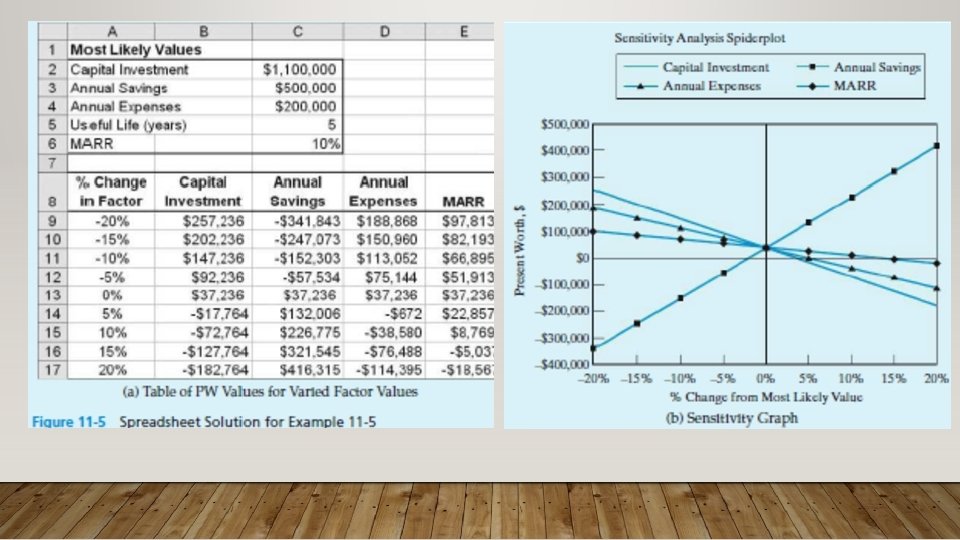
EXAMPLE 11 -5 Spiderplot for the Proposed Vision System We will now further explore the sensitivity of the proposed vision system by creating a spider plot. The best (most likely) estimates for the vision system described in Example 11 -4 are listed below. Capital investment, I RM 1, 100, 000 Annual savings, A 500, 000 Annual expenses, E 200, 000 MARR 10% We are interested in investigating the sensitivity of the PW of the system over a range of ± 20% changes in all of the above estimates. Recall that the useful life of the system is five years. Spreadsheet Solution Figure 11 -5(a) shows the table of PW values as each factor of the PW calculations is varied over a range of ± 20% from the most likely estimate. Each column has a unique formula that refers to the factors located in the range C 2: C 6 to determine PW. The particular factor of interest—for example, the capital investment in column B—is multiplied by the factor (1+percent change as a decimal) to create the table. You can verify your formulas by noting that all columns are equal at the most likely value (percent change = 0). The cell formulas in the range B 9: E 9 (listed below) are simply copied down the columns to complete the spreadsheet

The spider plot in Figure 11 -5(b) shows the sensitivity of the PW to percent deviation changes in each factor’s best estimate. The other factors are assumed to remain at their most likely values. The PW of this project based on the best estimates of the factors is PW(10%) = −RM 1, 100, 000 + (RM 500, 000 − RM 200, 000)(P/A, 10%, 5) = RM 37, 236. This value of the highly favorable PW occurs at the common intersection point of the percent deviation graphs for the four separate project factors. The relative degree of sensitivity of the PW to each factor is indicated by the slope of the curves (the steeper the slope of a curve the more sensitive the PW is to the factor). Also, the intersection of each curve with the abscissa (PW=0) shows the decision reversal point—the percent change from each factor’s most likely value at which the PW is zero. Based on the spiderplot, we see that the PW is insensitive to the MARR but quite sensitive to changes in the capital investment, annual savings, and annual expenses. Such an analytical tool as the spiderplot can assist with the insightful exploration of the variable aspects of an engineering economy study.

LEASE, BUY AND STATUS QUO DECISION • Leasing of assets is a business arrangement that makes assets available without incurring initial capital investment costs of purchase. • Lease specifications are generally detailed in a formal written contract.

EXAMPLE 13 -4 After-Tax Analysis: Buy, Lease, or Status Quo Suppose a firm is considering purchasing equipment for RM 200, 000 that would last for five years and have zero market value. Alternatively, the same equipment could be leased for RM 52, 000 at the beginning of each of those five years. The effective income tax rate for the firm is 55% and straight-line depreciation is used. The net before-tax cash benefits from the equipment are RM 56, 000 at the end of each year for five years. If the after-tax MARR for the firm is 10%, use the PW method to show whether the firm should buy, lease, or maintain the status quo. (A) (C ) = A - B (D) = -55% x C (E) = A + D (B) Alternative Year Before Taxable Cash Flow for After Tax Depreciation Cash Flow Income Tax Cash Flow Buy 0 -RM 200, 000 1– 5 Lease Status Quo -RM 200, 000 -RM 40, 000 +RM 22, 000 0 -RM 52, 000 +RM 28, 000 -RM 23, 000 1– 5 -RM 52, 000 +RM 28, 000 -RM 23, 000 1 -5 -RM 56, 000 +RM 30, 000 -RM 25, 000

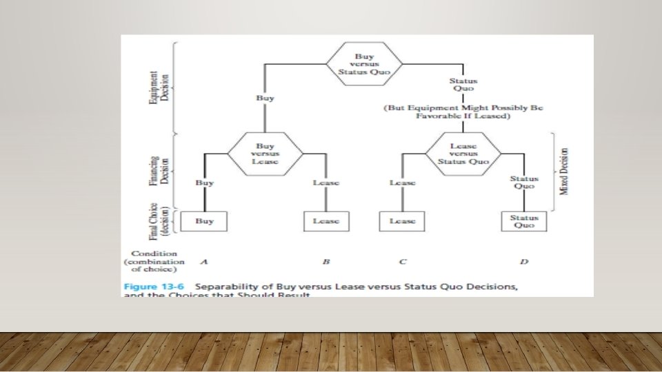
Thus, the PWs (after taxes) for the three alternatives are as follows: Buy: −RM 200, 000 + RM 22, 000(P/A, 10%, 5) = −RM 116, 600. Lease: −RM 23, 400 − RM 23, 400(P/A, 10%, 4) = −RM 97, 600. Status quo: −RM 25, 200(P/A, 10%, 5) = −RM 95, 500. We would first compare buy (PW = −RM 116, 600) against status quo (PW = −RM 95, 500) and find the status quo to be better. Then we would compare lease (PW = −RM 97, 600) against status quo (PW = −RM 95, 500) and find the status quo to be better. Thus, status quo is the better final choice. It should be noted that, had we merely compared buy versus lease, lease would have been the choice. But the final decision should not have been made without comparison against status quo.