Semivariogram Analysis and Estimation Tanya Nick Caroline Semivariogram

Semivariogram Analysis and Estimation Tanya, Nick Caroline

Semivariogram • • Gives information about the nature and structure of spatial dependency in a random field → must be estimated from the data Estimating a semivariogram: 1. 2. Derive empirical estimate from data Fit theoretical semivariogram model to empirical estimate

Properties • • • Evenness Passes through the origin Conditionally negative-definite

Second order stationary Random Field • Sill – upper asymptote • Range – distance at which semivariogram meets asymptote → covariance = zero • Observations spatially separated by more than the range are uncorrelated • Spatial autocorrelation exists only for pairs of points separated by less than the range • The more quickly semivariogram rises from the origin to the sill, the more quickly autocorrelation declines

Intrinsically but not second order stationary random field • Semivariogram never reaches upper asymptote • No range defined increase of semivariogram cannot be arbitrary

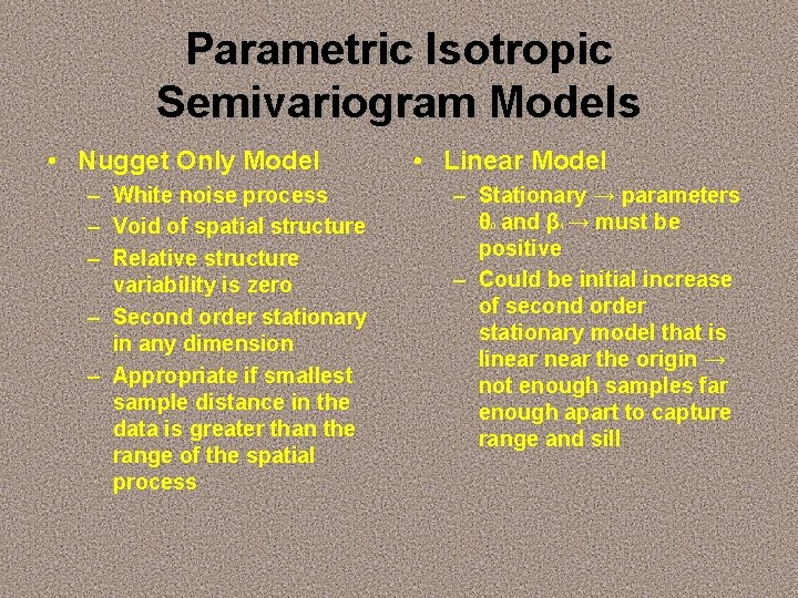
Parametric Isotropic Semivariogram Models • Nugget Only Model – – – White noise process Void of spatial structure Relative structure variability is zero – Second order stationary in any dimension – Appropriate if smallest sample distance in the data is greater than the range of the spatial process • Linear Model – Stationary → parameters θ and β → must be positive – Could be initial increase of second order stationary model that is linear the origin → not enough samples far enough apart to capture range and sill 0 1

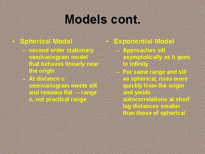
Models cont. • Spherical Model – second order stationary semivariogram model that behaves linearly near the origin – At distance α semivariogram meets sill and remains flat → range α, not practical range • Exponential Model – Approaches sill asymptotically as h goes to infinity – For same range and sill as spherical, rises more quickly from the origin and yields autocorrelations at short lag distances smaller than those of spherical

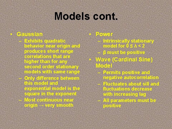
Models cont. • Gaussian – Exhibits quadratic behavior near origin and produces short range correlations that are higher than for any second order stationary models with same range – Only difference between this model and exponential model is the square in the exponent – Most continuous near origin → very smooth • Power – Intrinsically stationary model for 0 ≤ λ < 2 – β must be positive • Wave (Cardinal Sine) Model – Permits positive and negative autocorrelation – Fluctuates about sill and fluctuations decrease with increasing lag – All parameters must be positive

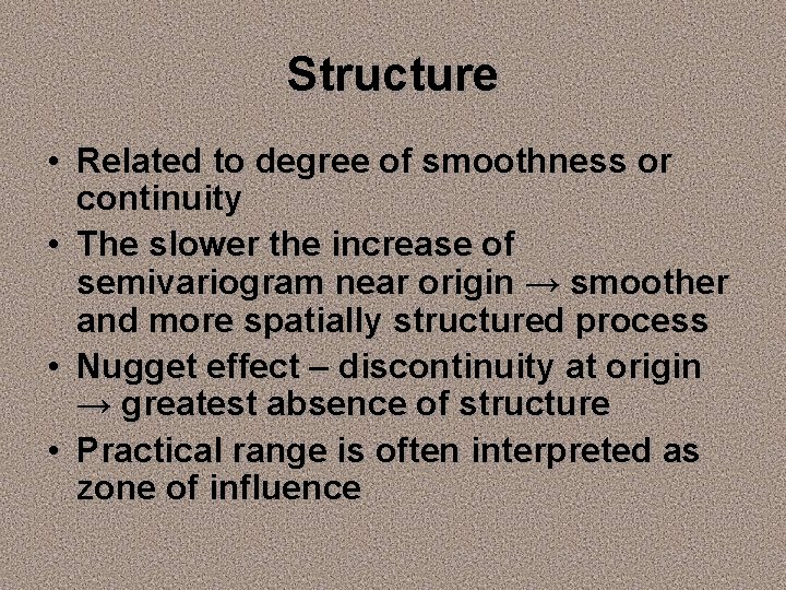
Structure • Related to degree of smoothness or continuity • The slower the increase of semivariogram near origin → smoother and more spatially structured process • Nugget effect – discontinuity at origin → greatest absence of structure • Practical range is often interpreted as zone of influence

Estimation and Fitting • Empirical Semivariogram estimators • Methods of Fitting: – Least squares – Maximum Likelihood – Composite Likelihood

Fitting by Least Squares • OLS requires data points to be uncorrelated and homoscedastic • Values of robust estimator are less correlated than those of Matheron estimator • Problem with generalized least squares approach → determination of variance – covariance matrix V

Fitting by Maximum Likelihood • Requires knowledge of distribution of the data • Data assumed to be Gaussian • Negatively biased • Has asymptotic efficiency

Composite Likelihood • Fairly new idea, only 10 years old • We have n Random variables • Uses Log Likelihood to Maximize • Calculated using computing power

Nested Models and Nonparametric Fitting • Non-Parametric models have one solid advantage • There could be a model inside one of the already known models, this is known as nesting • We start with a general model and see if we can find a model nested inside there

Homework • How many parametric semivariogram models are there and what are they? • What is the nugget effect? • List the different fitting methods. • Good luck on finals and have a great summer!!!