Seminar on random walks on graphs Lecture No

Seminar on random walks on graphs Lecture No. 2 Mille Gandelsman, 9. 11. 2009

Contents • Reversible and non-reversible Markov Chains. • Difficulty of sampling “simple to describe” distributions. • The Boolean cube. • The hard-core model. • The q-coloring problem. • MCMC and Gibbs samplers. • Fast convergence of Gibbs sampler for the Boolean cube. • Fast convergence of Gibbs sampler for random qcolorings.

Reminder A Markov chain with state space is said to be irreducible if for all we have that . A Markov chain with transition matrix is said to be aperiodic if for every there is an such that for every : Every irreducible and aperiodic Markov chain has exactly one stationary distribution.

Reversible Markov Chains • Definition: let be a Markov chain with state space and transition matrix. A probability distribution is said to be reversible for the chain (or for the transition matrix) if for all we have: • Definition: A Markov chain is said to be reversible if there exists a reversible distribution for it.

Reversible Markov Chains (cont. ) Theorem [HAG 6. 1]: let be a Markov chain with state space and transition matrix . If is a reversible distribution for the chain, then it is also a stationary distribution. Proof:

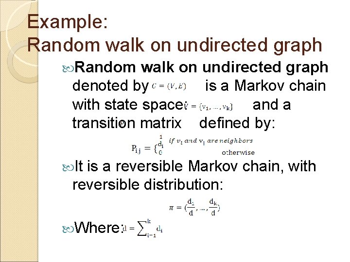
Example: Random walk on undirected graph denoted by is a Markov chain with state space: and a transition matrix defined by: It is a reversible Markov chain, with reversible distribution: Where:

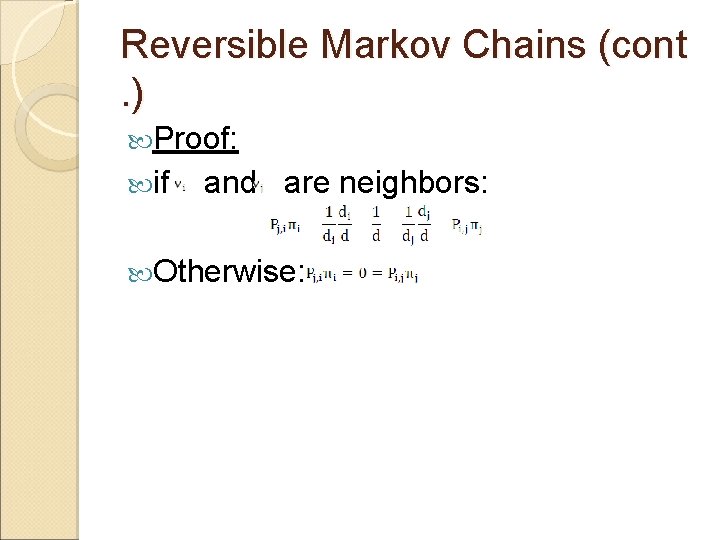
Reversible Markov Chains (cont . ) Proof: if and are neighbors: Otherwise:

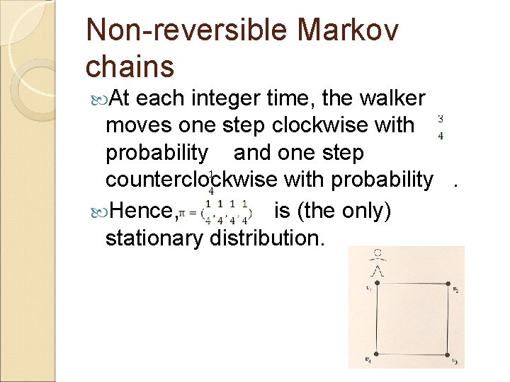
Non-reversible Markov chains At each integer time, the walker moves one step clockwise with probability and one step counterclockwise with probability . Hence, is (the only) stationary distribution.

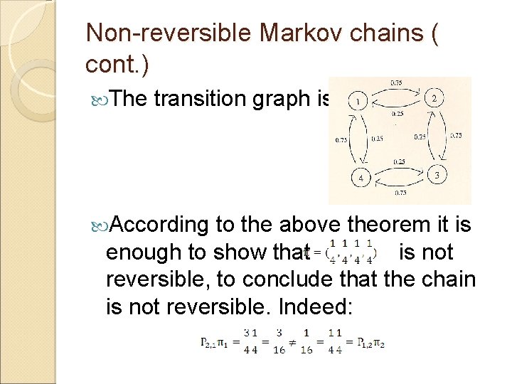
Non-reversible Markov chains ( cont. ) The transition graph is: According to the above theorem it is enough to show that is not reversible, to conclude that the chain is not reversible. Indeed:

Examples of distributions we would like to sample Boolean cube. The hard-core model. Q-coloring.

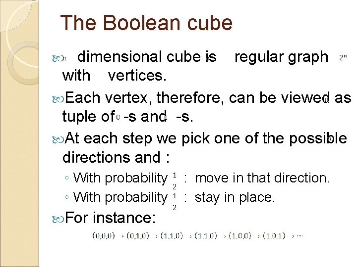
The Boolean cube dimensional cube is regular graph with vertices. Each vertex, therefore, can be viewed as tuple of -s and -s. At each step we pick one of the possible directions and : ◦ With probability : move in that direction. ◦ With probability : stay in place. For instance:

The Boolean cube (cont. ) What is the stationary distribution? How do we sample?

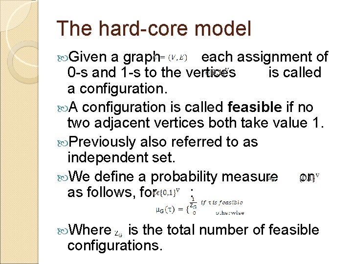
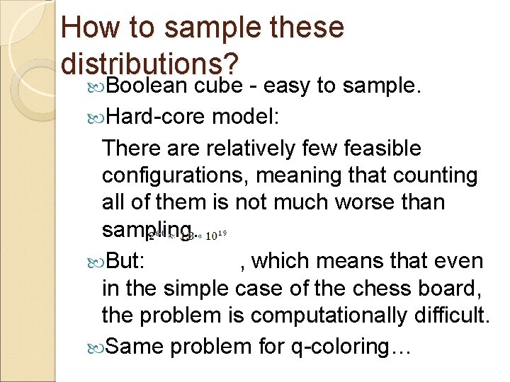
The hard-core model Given a graph each assignment of 0 -s and 1 -s to the vertices is called a configuration. A configuration is called feasible if no two adjacent vertices both take value 1. Previously also referred to as independent set. We define a probability measure on as follows, for : Where is the total number of feasible configurations.

The hard-core model (cont. ) An example of a random configuration chosen according to in the case where is the a square grid 8*8:

How to sample these distributions? Boolean cube - easy to sample. Hard-core model: There are relatively few feasible configurations, meaning that counting all of them is not much worse than sampling. But: , which means that even in the simple case of the chess board, the problem is computationally difficult. Same problem for q-coloring…

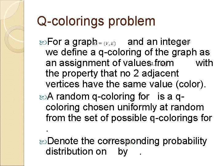
Q-colorings problem For a graph and an integer we define a q-coloring of the graph as an assignment of values from with the property that no 2 adjacent vertices have the same value (color). A random q-coloring for is a qcoloring chosen uniformly at random from the set of possible q-colorings for . Denote the corresponding probability distribution on by .

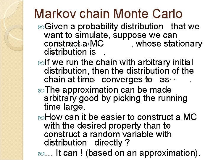
Markov chain Monte Carlo Given a probability distribution that we want to simulate, suppose we can construct a MC , whose stationary distribution is . If we run the chain with arbitrary initial distribution, then the distribution of the chain at time converges to as . The approximation can be made arbitrary good by picking the running time large. How can it be easier to construct a MC with the desired property than to construct a random variable with distribution directly ? … It can ! (based on an approximation).

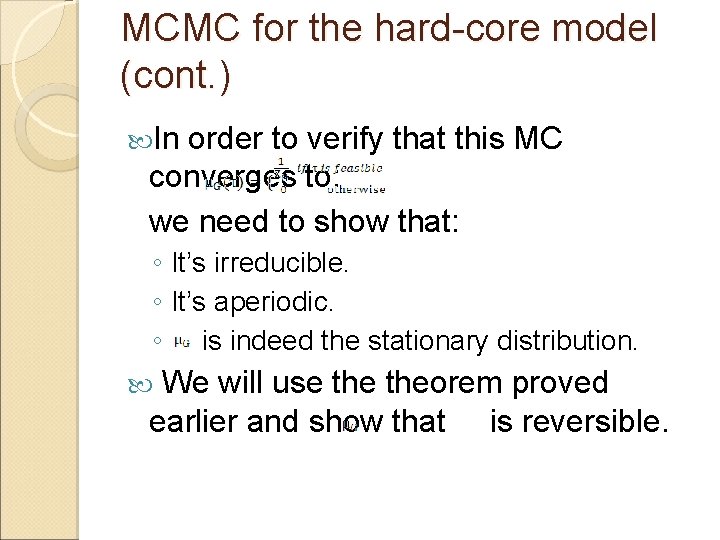
MCMC for the hard-core model Let us define a MC whose state space is given by: , with the following transition mechanism - at each integer time , we do as follows: ◦ Pick a vertex uniformly at random. ◦ With probability : if all the neighbors of take the value 0 in then let: Otherwise: ◦ For all vertices other than :

MCMC for the hard-core model (cont. ) In order to verify that this MC converges to: we need to show that: ◦ It’s irreducible. ◦ It’s aperiodic. ◦ is indeed the stationary distribution. We will use theorem proved earlier and show that is reversible.

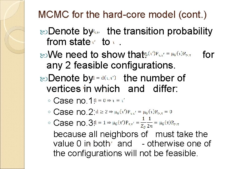
MCMC for the hard-core model (cont. ) Denote by the transition probability from state to . We need to show that: for any 2 feasible configurations. Denote by the number of vertices in which and differ: ◦ Case no. 1: ◦ Case no. 2: ◦ Case no. 3: because all neighbors of must take the value 0 in both and - otherwise one of the configurations will not be feasible.

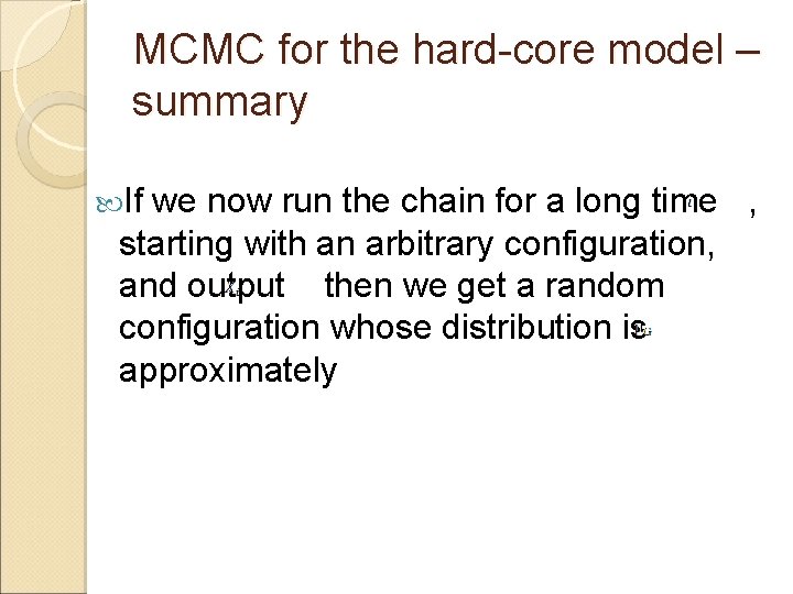
MCMC for the hard-core model – summary If we now run the chain for a long time , starting with an arbitrary configuration, and output then we get a random configuration whose distribution is approximately

MCMC and Gibbs Samplers Note: We found a distribution that is reversible, though it is only required that it will be stationary. This is often the case because it is an easy way to find a stationary distribution. The above algorithm is an example of a special class of MCMC algorithms known Gibbs Samplers.

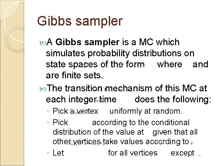
Gibbs sampler A Gibbs sampler is a MC which simulates probability distributions on state spaces of the form where and are finite sets. The transition mechanism of this MC at each integer time does the following: ◦ Pick a vertex uniformly at random. ◦ Pick according to the conditional distribution of the value at given that all other vertices take values according to ◦ Let for all vertices except .