Seminar on Dynamic Programming Background Algorithms An algorithm

Seminar on Dynamic Programming

Background Algorithms An algorithm is a sequence of unambiguous instructions for solving a problem, i. e. , for obtaining a required output for any legitimate input in a finite amount of time.

Classifications Algorithms can be classified in numerous ways: Design Techniques and Efficiency.

Design Techniques Brute Force Divide and Conquer Decrease and Conquer Transform and conquer Space-Time Tradeoffs Greedy Technique Dynamic Programming Iterative improvement Backtracking Branch and bound

Dynamic Programming Invented by American mathematician Richard Bellman in the 1950 s’ to solve optimization problems and later assimilated by CS. Dynamic Programming is a general algorithm design technique for solving problems with overlapping subproblems.

Dynamic Programming Used for optimization problems A set of choices must be made to get an optimal solution Find a solution with the optimal value (minimum or maximum) There may be many solutions that lead to an optimal value Our goal: find an optimal solution

Examples of DP algorithms Computing a binomial coefficient. Knapsack problem Matrix-Chain Multiplication

Computing a binomial coefficient. Binomial coefficients are coefficients of the binomial formula: (a + b)n = C(n, 0)anb 0 +. . . + C(n, k)an-kbk +. . . + C(n, n)a 0 bn Properties : C(n, k) = C(n-1, k) + C(n-1, k-1) for n > k > 0 C(n, 0) = 1, C(n, n) = 1 for n 0

Computing C(n, k): pseudocode

Value of C(n, k) can be computed by filling a table:

Knapsack problem There are two versions of the problem: “ 0 -1 knapsack problem” Items are indivisible; you either take an item or not. Solved with dynamic programming. “Fractional knapsack problem” Items are divisible: you can take any fraction of an item. Solved with a greedy algorithm.

Knapsack Problem by DP Given n items of integer weights: values: w 1 w 2 … w n v 1 v 2 … v n a knapsack of integer capacity W find most valuable subset of the items that fit into the knapsack Consider instance defined by first i items and capacity j (j W). Let V[i, j] be optimal value of such instance. Then max {V[i-1, j], vi + V[i-1, j- wi]} if j- wi 0 V[i, j] = V[i-1, j] if j- wi < 0 Initial conditions: V[0, j] = 0 and V[i, 0] = 0

Knapsack problem

Example i 0 0 0 1 0 2 0 3 0 4 0 1 2 3 4 5

Example i 0 0 0 1 0 2 0 3 0 4 5 0 0

Matrix-Chain Multiplication Problem: given a sequence A 1, A 2, …, An , compute the product: A 1 A 2 An Matrix compatibility: C=A B

MATRIX-MULTIPLY(A, B) if columns[A] rows[B] then error “incompatible dimensions” else for i 1 to rows[A] do for j 1 to columns[B] do C[i, j] = 0 for k 1 to columns[A] do C[i, j] + A[i, k] B[k, j]

Matrix-Chain Multiplication In what order should we multiply the matrices? A 1 A 2 An Parenthesize the product to get the order in which matrices are multiplied E. g. : A 1 A 2 A 3 = ((A 1 A 2) A 3) = (A 1 (A 2 A 3)) Which one of these orderings should we choose? The order in which we multiply the matrices has a significant impact on the cost of evaluating the product

Example A 1 A 2 A 3 A 1: 10 x 100 A 2: 100 x 5 A 3: 5 x 50 1. ((A 1 A 2) A 3): A 1 A 2 = 10 x 100 x 5 = 5, 000 (10 x 5) ((A 1 A 2) A 3) = 10 x 50 = 2, 500 Total: 7, 500 scalar multiplications 2. (A 1 (A 2 A 3)): A 2 A 3 = 100 x 50 = 25, 000 (100 x 50) (A 1 (A 2 A 3)) = 10 x 100 x 50 = 50, 000 Total: 75, 000 scalar multiplications one order of magnitude difference!!

Matrix-Chain Multiplication: Problem Statement Given a chain of matrices A 1, A 2, …, An , where Ai has dimensions pi-1 x pi, fully parenthesize the product A 1 A 2 An in a way that minimizes the number of scalar multiplications. A 1 p 0 x p 1 A 2 p 1 x p 2 Ai pi-1 x pi Ai+1 pi x pi+1 An pn-1 x pn

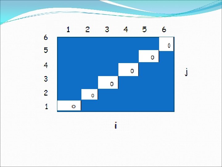
Computing the Optimal Costs 0 if i = j m[i, j] = min {m[i, k] + m[k+1, j] + pi-1 pkpj} if i < j i k<j Length = 1: i = j, i = 1, 2, …, n Length = 2: j = i + 1, i = 1, 2, …, n-1 m[1, n] gives the optimal solution to the problem Compute rows from bottom to top and from left to right n 3 2 1 1 2 3 n

Example: min {m[i, k] + m[k+1, j] + pi-1 pkpj} m[2, 2] + m[3, 5] + p 1 p 2 p 5 m[2, 3] + m[4, 5] + p 1 p 3 p 5 m[2, 4] + m[5, 5] + p 1 p 4 p 5 m[2, 5] = min 1 2 3 4 5 k=2 k=3 k=4 6 6 5 4 j 3 2 1 i • Values m[i, j] depend only on values that have been previously computed

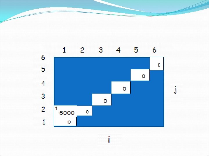
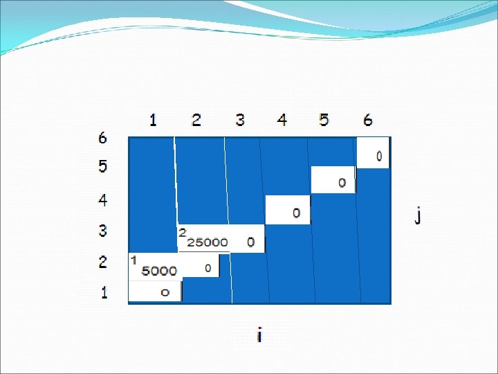
Example min {m[i, k] + m[k+1, j] + pi-1 pkpj} Compute A 1 A 2 A 3 A 1: 10 x 100 (p 0 x p 1) A 2: 100 x 5 (p 1 x p 2) A 3: 5 x 50 (p 2 x p 3) m[i, i] = 0 for i = 1, 2, 3 m[1, 2] = m[1, 1] + m[2, 2] + p 0 p 1 p 2 (A 1 A 2) = 0 + 10 *100* 5 = 5, 000 m[2, 3] = m[2, 2] + m[3, 3] + p 1 p 2 p 3 (A 2 A 3) = 0 + 100 * 50 = 25, 000 m[1, 3] = min m[1, 1] + m[2, 3] + p 0 p 1 p 3 = 75, 000 (A 1(A 2 A 3)) m[1, 2] + m[3, 3] + p 0 p 2 p 3 = 7, 500 ((A 1 A 2)A 3)

Matrix-Chain-Order(p)