Semidynamic compact index for short patterns and succinct

Semi-dynamic compact index for short patterns and succinct van Emde Boas tree Yoshiaki Matsuoka 1, Tomohiro I 2, Shunsuke Inenaga 1, Hideo Bannai 1, Masayuki Takeda 1 (1 Kyushu University) (2 TU Dortmund) 1

Overview Ø There exist many space-efficient indices (e. g. FM-index [Ferragina&Manzini, 2000]) but most of them are static. Ø Some (e. g. Dynamic FM-index [Salson et al. , 2010]) are dynamic but consume more space than static counterparts. 2

Overview Ø There exist many space-efficient indices (e. g. FM-index [Ferragina&Manzini, 2000]) but most of them are static. Ø Some (e. g. Dynamic FM-index [Salson et al. , 2010]) are dynamic but consume more space than static counterparts. Ø We propose a self-index for searching patterns of limited length, which: • is theoretically and practically efficient in terms of construction, updates (adding characters at the end of the text) and searches, • is compact, i. e. , requires only O(n log σ) bits of space, where n is the text size and σ is the alphabet size, and • can be constructed in online manner. 3

Problem Ø Preprocess : text T of length n over an alphabet of size σ. Ø Query : pattern P of length at most r. Ø Answer : all occurrences of P in T. 4

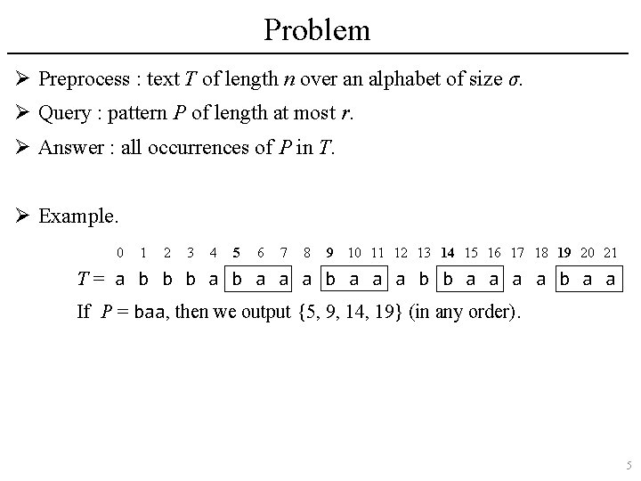
Problem Ø Preprocess : text T of length n over an alphabet of size σ. Ø Query : pattern P of length at most r. Ø Answer : all occurrences of P in T. Ø Example. 0 1 2 3 4 5 6 7 8 9 10 11 12 13 14 15 16 17 18 19 20 21 T= a b b b a a a b b a a If P = baa, then we output {5, 9, 14, 19} (in any order). 5

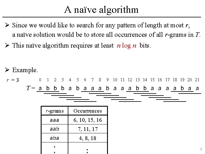
A naïve algorithm Ø Since we would like to search for any pattern of length at most r, a naïve solution would be to store all occurrences of all r-grams in T. Ø This naïve algorithm requires at least n log n bits. Ø Example. r =3 0 1 2 3 4 5 6 7 8 9 10 11 12 13 14 15 16 17 18 19 20 21 T= a b b b a a a b b a a r-grams Occurrences aaa 6, 10, 15, 16 aab 7, 11, 17 aba 4, 8, 18 ・・ ・・ 6

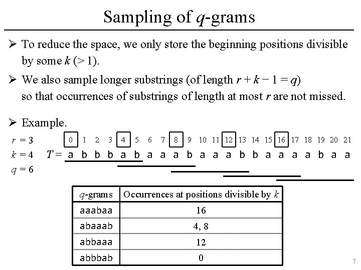
Sampling of q-grams Ø To reduce the space, we only store the beginning positions divisible by some k (> 1). Ø We also sample longer substrings (of length r + k − 1 = q) so that occurrences of substrings of length at most r are not missed. Ø Example. r =3 k=4 q=6 0 1 2 3 4 5 6 7 8 9 10 11 12 13 14 15 16 17 18 19 20 21 T= a b b b a a a b b a a q-grams Occurrences at positions divisible by k aaabaa 16 abaaab 4, 8 abbaaa 12 abbbab 0 7

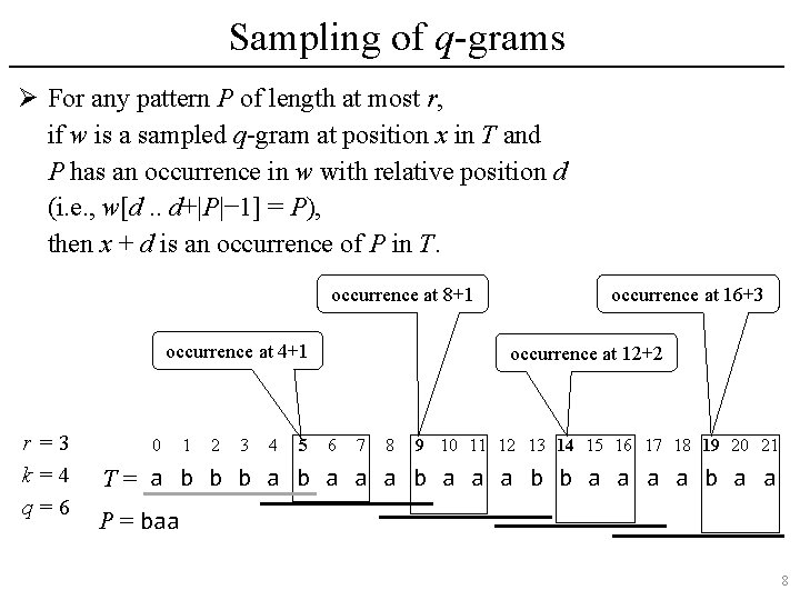
Sampling of q-grams Ø For any pattern P of length at most r, if w is a sampled q-gram at position x in T and P has an occurrence in w with relative position d (i. e. , w[d. . d+|P|− 1] = P), then x + d is an occurrence of P in T. occurrence at 8+1 occurrence at 4+1 r =3 k=4 q=6 0 1 2 3 4 5 occurrence at 16+3 occurrence at 12+2 6 7 8 9 10 11 12 13 14 15 16 17 18 19 20 21 T= a b b b a a a b b a a P = baa 8

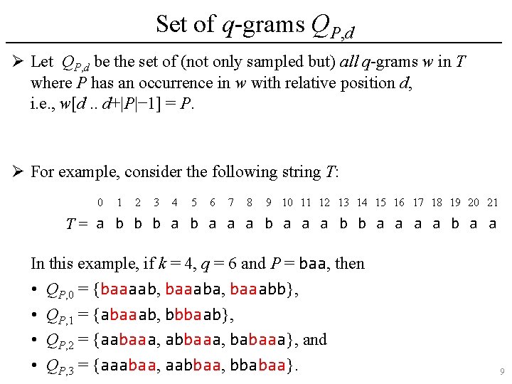
Set of q-grams QP, d Ø Let QP, d be the set of (not only sampled but) all q-grams w in T where P has an occurrence in w with relative position d, i. e. , w[d. . d+|P|− 1] = P. Ø For example, consider the following string T: 0 1 2 3 4 5 6 7 8 9 10 11 12 13 14 15 16 17 18 19 20 21 T= a b b b a a a b b a a In this example, if k = 4, q = 6 and P = baa, then • QP, 0 = {baaaab, baaaba, baaabb}, • QP, 1 = {abaaab, bbbaab}, • QP, 2 = {aabaaa, abbaaa, babaaa}, and • QP, 3 = {aaabaa, aabbaa, bbabaa}. 9

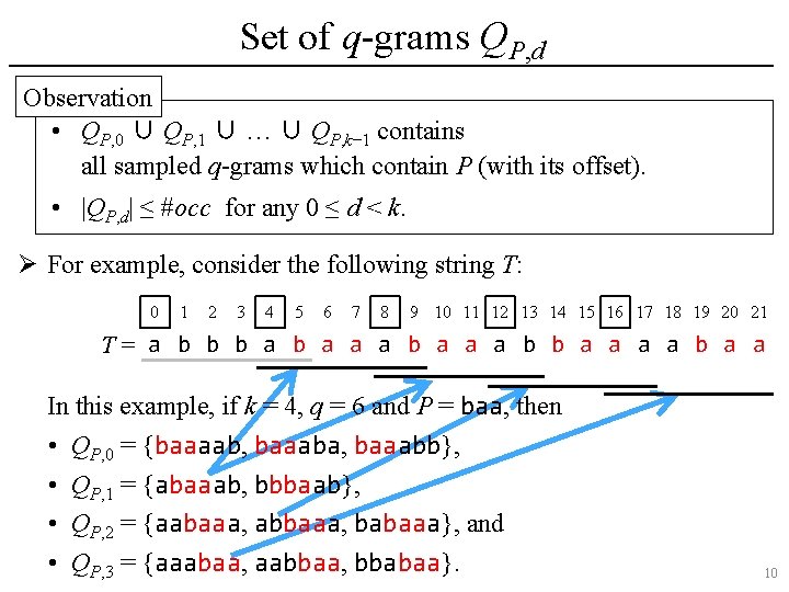
Set of q-grams QP, d Ø Observation • QP, 0 ∪ QP, 1 ∪ … ∪ QP, k− 1 contains all sampled q-grams which contain P (with its offset). • |QP, d| ≤ #occ for any 0 ≤ d < k. Ø For example, consider the following string T: 0 1 2 3 4 5 6 7 8 9 10 11 12 13 14 15 16 17 18 19 20 21 T= a b b b a a a b b a a In this example, if k = 4, q = 6 and P = baa, then • QP, 0 = {baaaab, baaaba, baaabb}, • QP, 1 = {abaaab, bbbaab}, • QP, 2 = {aabaaa, abbaaa, babaaa}, and • QP, 3 = {aaabaa, aabbaa, bbabaa}. 10

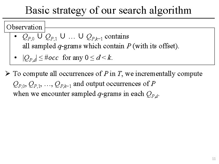
Basic strategy of our search algorithm Observation • QP, 0 ∪ QP, 1 ∪ … ∪ QP, k− 1 contains all sampled q-grams which contain P (with its offset). • |QP, d| ≤ #occ for any 0 ≤ d < k. Ø To compute all occurrences of P in T, we incrementally compute QP, 0, QP, 1, …, QP, k− 1 and output occurrences of P when we encounter sampled q-grams in each QP, d. 11

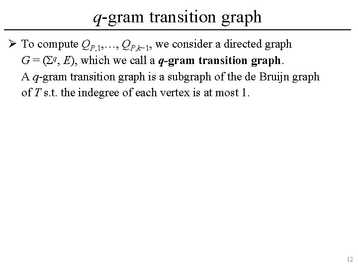
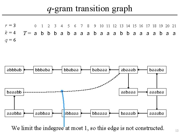
q-gram transition graph Ø To compute QP, 1, …, QP, k− 1, we consider a directed graph G = (Σq, E), which we call a q-gram transition graph. A q-gram transition graph is a subgraph of the de Bruijn graph of T s. t. the indegree of each vertex is at most 1. 12

q-gram transition graph r =3 k=4 q=6 abbbab 0 1 2 3 4 5 6 7 8 9 10 11 12 13 14 15 16 17 18 19 20 21 T= a b b b a a a b b a a bbbabaa babaaabb aaabbaa abbaaaa abaaaba aabaaa aaabaa baaaaba We limit the indegree at most 1, so this edge is not constructed. 13

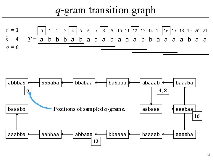
q-gram transition graph r =3 k=4 q=6 0 1 2 3 4 5 6 7 8 9 10 11 12 13 14 15 16 17 18 19 20 21 T= a b b b a a a b b a a abbbaba bbabaaa 0 baaabb Positions of sampled q-grams. abaaab 4, 8 baaabaaa aaabaa 16 aaabbaa abbaaaa baaaaba 12 14

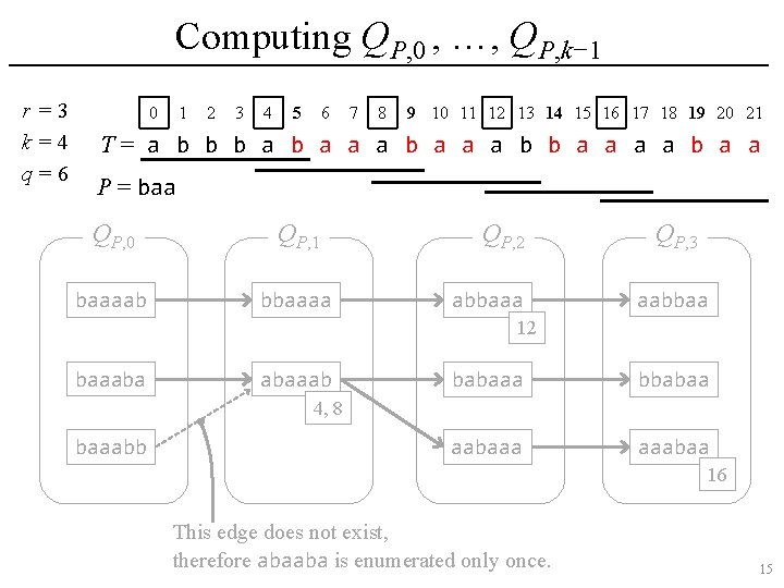
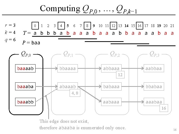
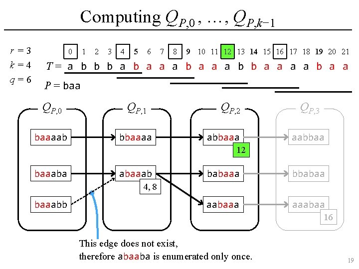
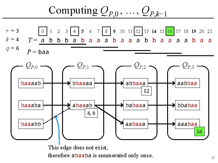
Computing QP, 0 , …, QP, k− 1 r =3 k=4 q=6 0 1 2 3 4 5 6 7 8 9 10 11 12 13 14 15 16 17 18 19 20 21 T= a b b b a a a b b a a P = baa QP, 0 QP, 1 baaaab bbaaaa QP, 2 abbaaa QP, 3 aabbaa 12 baaaba abaaab babaaa bbabaa aabaaa aaabaa 4, 8 baaabb 16 This edge does not exist, therefore abaaba is enumerated only once. 15

Computing QP, 0 , …, QP, k− 1 r =3 k=4 q=6 0 1 2 3 4 5 6 7 8 9 10 11 12 13 14 15 16 17 18 19 20 21 T= a b b b a a a b b a a P = baa QP, 0 QP, 1 baaaab bbaaaa QP, 2 abbaaa QP, 3 aabbaa 12 baaaba abaaab babaaa bbabaa aabaaa aaabaa 4, 8 baaabb 16 This edge does not exist, therefore abaaba is enumerated only once. 16

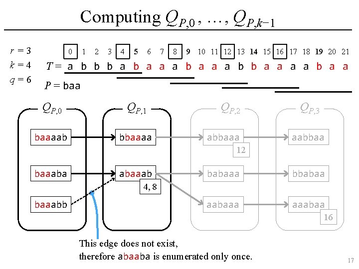
Computing QP, 0 , …, QP, k− 1 r =3 k=4 q=6 0 1 2 3 4 5 6 7 8 9 10 11 12 13 14 15 16 17 18 19 20 21 T= a b b b a a a b b a a P = baa QP, 0 QP, 1 baaaab bbaaaa QP, 2 abbaaa QP, 3 aabbaa 12 baaaba abaaab babaaa bbabaa aabaaa aaabaa 4, 8 baaabb 16 This edge does not exist, therefore abaaba is enumerated only once. 17

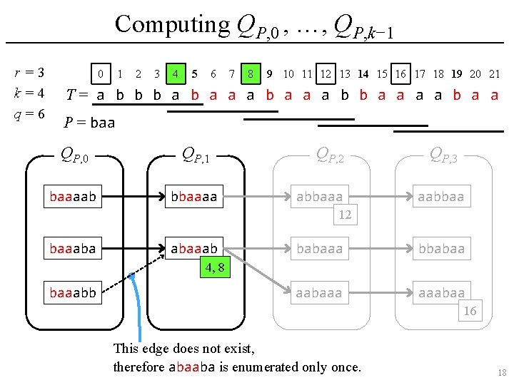
Computing QP, 0 , …, QP, k− 1 r =3 k=4 q=6 0 1 2 3 4 5 6 7 8 9 10 11 12 13 14 15 16 17 18 19 20 21 T= a b b b a a a b b a a P = baa QP, 0 QP, 1 baaaab bbaaaa QP, 2 abbaaa QP, 3 aabbaa 12 baaaba abaaab babaaa bbabaa aabaaa aaabaa 4, 8 baaabb 16 This edge does not exist, therefore abaaba is enumerated only once. 18

Computing QP, 0 , …, QP, k− 1 r =3 k=4 q=6 0 1 2 3 4 5 6 7 8 9 10 11 12 13 14 15 16 17 18 19 20 21 T= a b b b a a a b b a a P = baa QP, 0 QP, 1 baaaab bbaaaa QP, 2 abbaaa QP, 3 aabbaa 12 baaaba abaaab babaaa bbabaa aabaaa aaabaa 4, 8 baaabb 16 This edge does not exist, therefore abaaba is enumerated only once. 19

Computing QP, 0 , …, QP, k− 1 r =3 k=4 q=6 0 1 2 3 4 5 6 7 8 9 10 11 12 13 14 15 16 17 18 19 20 21 T= a b b b a a a b b a a P = baa QP, 0 QP, 1 baaaab bbaaaa QP, 2 abbaaa QP, 3 aabbaa 12 baaaba abaaab babaaa bbabaa aabaaa aaabaa 4, 8 baaabb 16 This edge does not exist, therefore abaaba is enumerated only once. 20

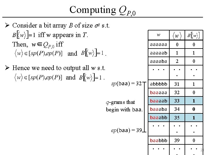
Computing QP, 0 Ø Given pattern P, first we need to compute the source QP, 0 of the q-gram transition graph, i. e. , all q-grams in T which begin with P. 21

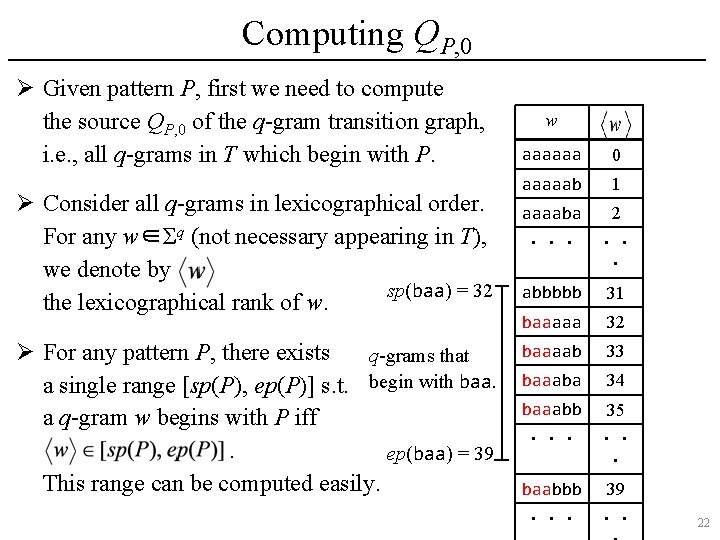
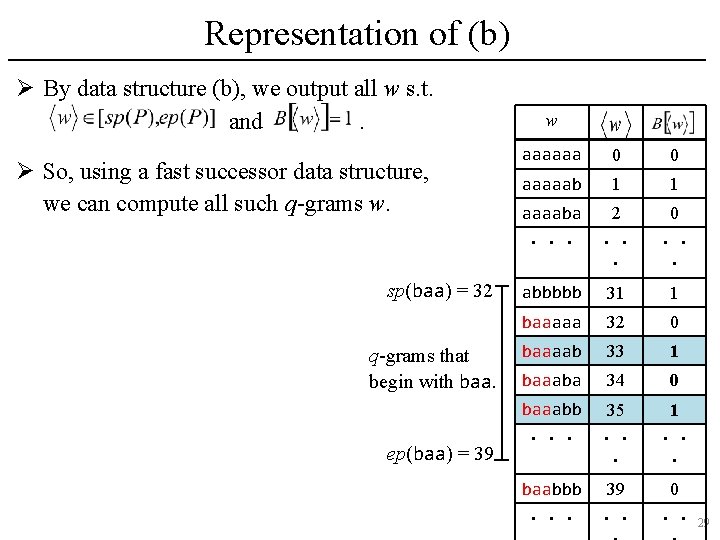
Computing QP, 0 Ø Given pattern P, first we need to compute the source QP, 0 of the q-gram transition graph, i. e. , all q-grams in T which begin with P. Ø Consider all q-grams in lexicographical order. For any w∈Σq (not necessary appearing in T), we denote by sp(baa) = 32 the lexicographical rank of w. Ø For any pattern P, there exists q-grams that a single range [sp(P), ep(P)] s. t. begin with baa. a q-gram w begins with P iff. ep(baa) = 39 This range can be computed easily. w aaaaaa 0 aaaaab 1 aaaaba 2 ・・・ ・・ ・ abbbbb 31 baaaaa 32 baaaab 33 baaaba 34 baaabb 35 ・・・ ・・ ・ baabbb 39 ・・・ ・・ 22

Computing QP, 0 Ø Consider a bit array B of size σq s. t. iff w appears in T. Then, w∈QP, 0 iff and. Ø Hence we need to output all w s. t. and. w sp(baa) = 32 q-grams that begin with baa. ep(baa) = 39 aaaaaa 0 0 aaaaab 1 1 aaaaba 2 0 ・・・ ・・ ・ abbbbb 31 1 baaaaa 32 0 baaaab 33 1 baaaba 34 0 baaabb 35 1 ・・・ ・・ ・ baabbb 39 0 ・・・ ・・ ・・ 23

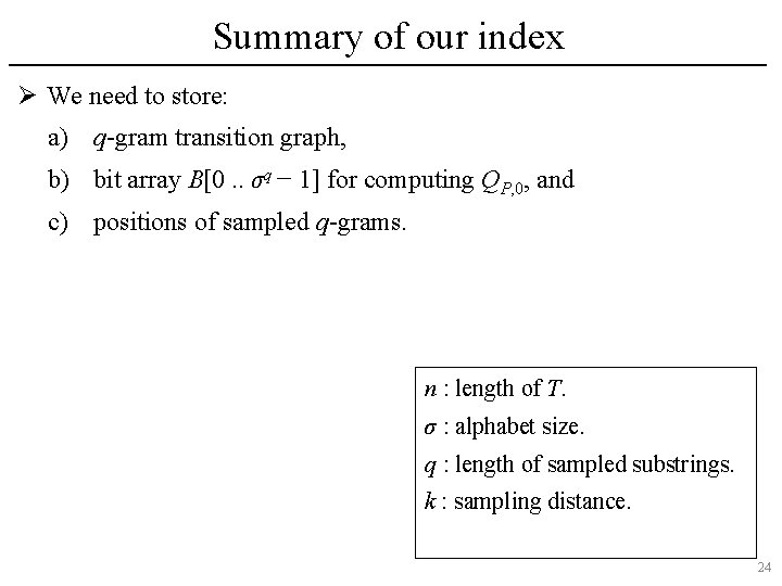
Summary of our index Ø We need to store: a) q-gram transition graph, b) bit array B[0. . σq − 1] for computing QP, 0, and c) positions of sampled q-grams. n : length of T. σ : alphabet size. q : length of sampled substrings. k : sampling distance. 24

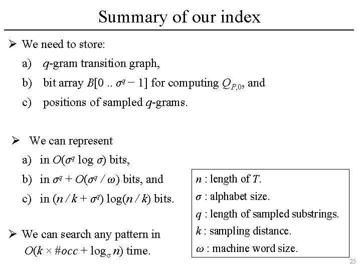
Summary of our index Ø We need to store: a) q-gram transition graph, b) bit array B[0. . σq − 1] for computing QP, 0, and c) positions of sampled q-grams. Ø We can represent a) in O(σq log σ) bits, b) in σq + O(σq / ω) bits, and n : length of T. c) in (n / k + σq) log(n / k) bits. σ : alphabet size. q : length of sampled substrings. Ø We can search any pattern in O(k × #occ + logσ n) time. k : sampling distance. ω : machine word size. 25

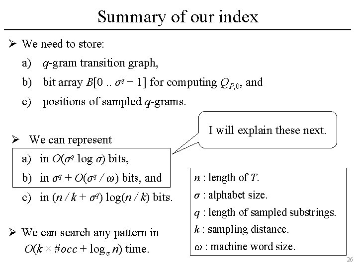
Summary of our index Ø We need to store: a) q-gram transition graph, b) bit array B[0. . σq − 1] for computing QP, 0, and c) positions of sampled q-grams. Ø We can represent I will explain these next. a) in O(σq log σ) bits, b) in σq + O(σq / ω) bits, and n : length of T. c) in (n / k + σq) log(n / k) bits. σ : alphabet size. q : length of sampled substrings. Ø We can search any pattern in O(k × #occ + logσ n) time. k : sampling distance. ω : machine word size. 26

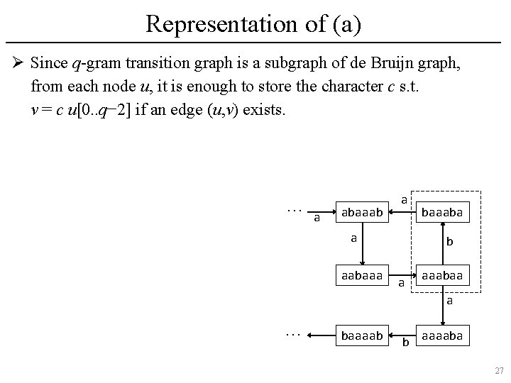
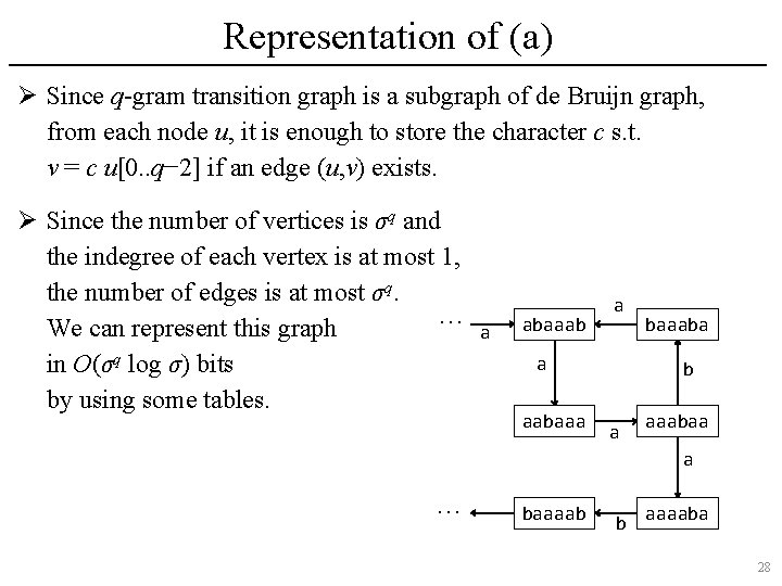
Representation of (a) Ø Since q-gram transition graph is a subgraph of de Bruijn graph, from each node u, it is enough to store the character c s. t. v = c u[0. . q− 2] if an edge (u, v) exists. … a abaaab a a aabaaaba b a aaabaa a … baaaab b aaaaba 27

Representation of (a) Ø Since q-gram transition graph is a subgraph of de Bruijn graph, from each node u, it is enough to store the character c s. t. v = c u[0. . q− 2] if an edge (u, v) exists. Ø Since the number of vertices is σq and the indegree of each vertex is at most 1, the number of edges is at most σq. … We can represent this graph in O(σq log σ) bits by using some tables. a abaaab a a aabaaaba b a aaabaa a … baaaab b aaaaba 28

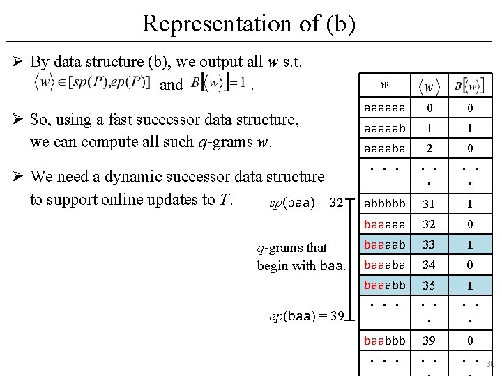
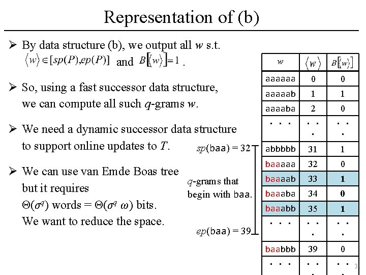
Representation of (b) Ø By data structure (b), we output all w s. t. and. Ø So, using a fast successor data structure, we can compute all such q-grams w. sp(baa) = 32 q-grams that begin with baa. ep(baa) = 39 w aaaaaa 0 0 aaaaab 1 1 aaaaba 2 0 ・・・ ・・ ・ abbbbb 31 1 baaaaa 32 0 baaaab 33 1 baaaba 34 0 baaabb 35 1 ・・・ ・・ ・ baabbb 39 0 ・・・ ・・ ・・ 29

Representation of (b) Ø By data structure (b), we output all w s. t. and. Ø So, using a fast successor data structure, we can compute all such q-grams w. Ø We need a dynamic successor data structure to support online updates to T. sp(baa) = 32 q-grams that begin with baa. ep(baa) = 39 w aaaaaa 0 0 aaaaab 1 1 aaaaba 2 0 ・・・ ・・ ・ abbbbb 31 1 baaaaa 32 0 baaaab 33 1 baaaba 34 0 baaabb 35 1 ・・・ ・・ ・ baabbb 39 0 ・・・ ・・ ・・ 30

Representation of (b) Ø By data structure (b), we output all w s. t. and. Ø So, using a fast successor data structure, we can compute all such q-grams w. Ø We need a dynamic successor data structure to support online updates to T. sp(baa) = 32 Ø We can use van Emde Boas tree q-grams that but it requires begin with baa. q q Θ(σ ) words = Θ(σ ω) bits. We want to reduce the space. ep(baa) = 39 w aaaaaa 0 0 aaaaab 1 1 aaaaba 2 0 ・・・ ・・ ・ abbbbb 31 1 baaaaa 32 0 baaaab 33 1 baaaba 34 0 baaabb 35 1 ・・・ ・・ ・ baabbb 39 0 ・・・ ・・ ・・ 31

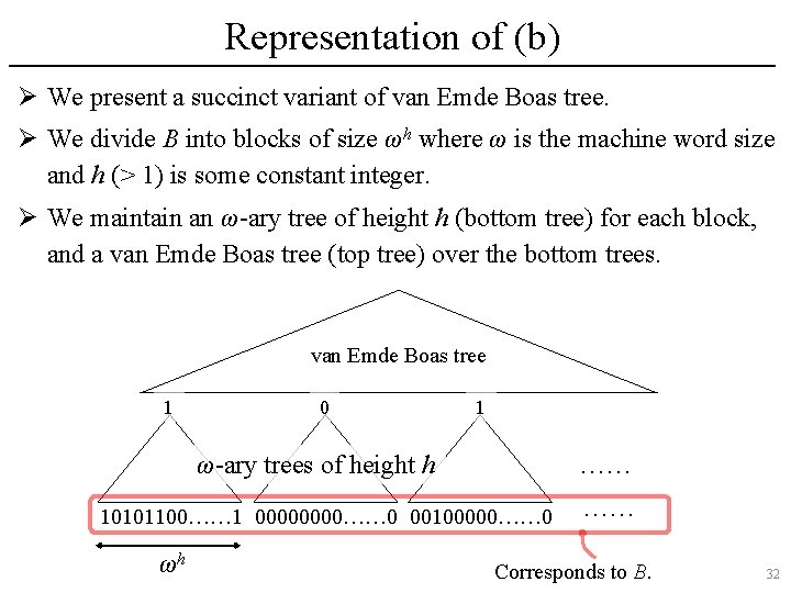
Representation of (b) Ø We present a succinct variant of van Emde Boas tree. Ø We divide B into blocks of size ωh where ω is the machine word size and h (> 1) is some constant integer. Ø We maintain an ω-ary tree of height h (bottom tree) for each block, and a van Emde Boas tree (top tree) over the bottom trees. van Emde Boas tree 1 0 1 ω-ary trees of height h …… 10101100…… 1 0000…… 0 00100000…… 0 ωh …… Corresponds to B. 32

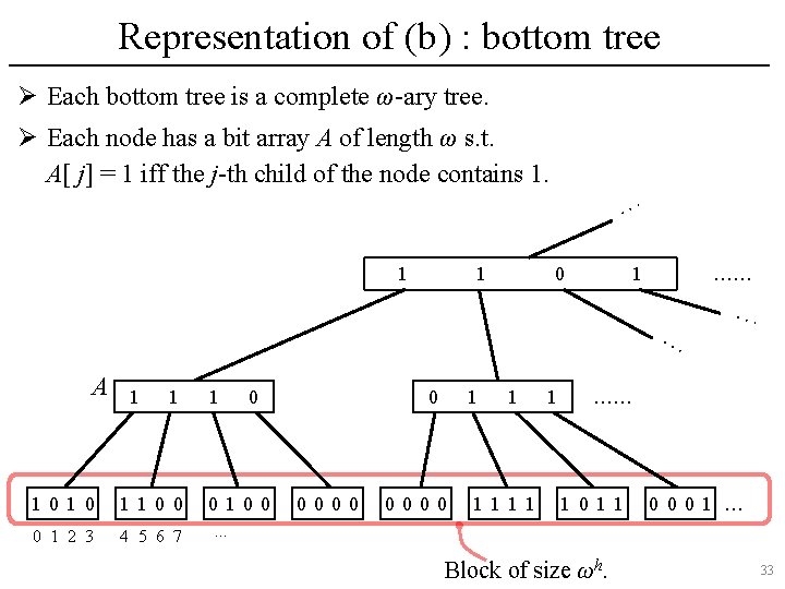
Representation of (b) : bottom tree Ø Each bottom tree is a complete ω-ary tree. Ø Each node has a bit array A of length ω s. t. A[ j] = 1 iff the j-th child of the node contains 1. … 1 1 0 1 …… … A 1 1 1010 1100 0 1 2 3 4 5 6 7 1 0 aaaaaaaa 0 0100 0000 1 1111 1 … …… 1011 0001 … . . . Block of size ωh. 33

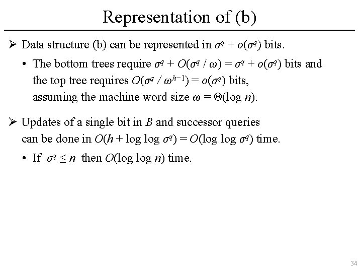
Representation of (b) Ø Data structure (b) can be represented in σq + o(σq) bits. • The bottom trees require σq + O(σq / ω) = σq + o(σq) bits and the top tree requires O(σq / ωh− 1) = o(σq) bits, assuming the machine word size ω = Θ(log n). Ø Updates of a single bit in B and successor queries can be done in O(h + log σq) = O(log σq) time. • If σq ≤ n then O(log n) time. 34

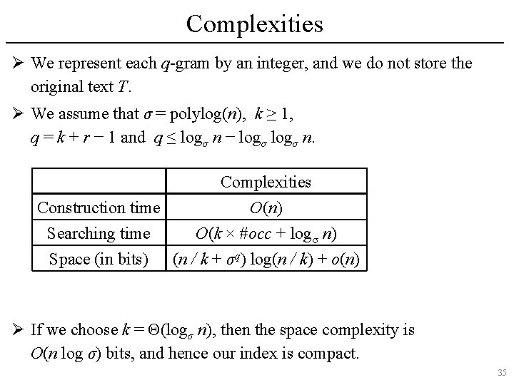
Complexities Ø We represent each q-gram by an integer, and we do not store the original text T. Ø We assume that σ = polylog(n), k ≥ 1, q = k + r − 1 and q ≤ logσ n − logσ n. Complexities Construction time O(n) Searching time O(k × #occ + logσ n) Space (in bits) (n / k + σq) log(n / k) + o(n) Ø If we choose k = Θ(logσ n), then the space complexity is O(n log σ) bits, and hence our index is compact. 35

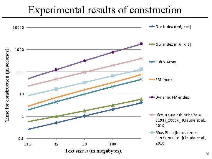
Experimental results of construction Our index (r=6, k=4) 10000 Time for construction (in seconds). Our index (r=6, k=6) 1000 Suffix Array 100 FM-index 10 Dynamic FM-index Rice, Re-Pair (block size = 8192)_x 000 d_[Claude et al. , 2010] 1 0. 1 12. 5 25 50 100 Text size n (in megabytes). Rice, Plain (block size = 8192)_x 000 d_[Claude et al. , 2010] 36

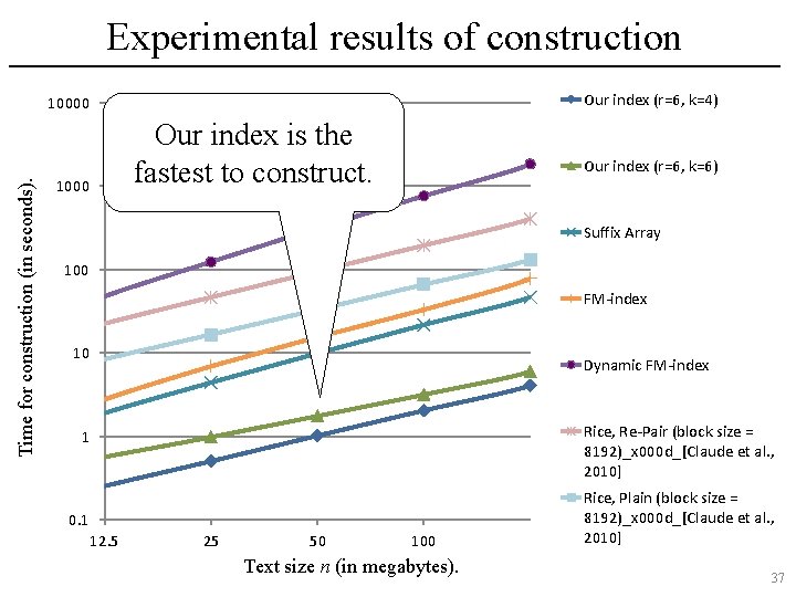
Experimental results of construction Our index (r=6, k=4) Time for construction (in seconds). 10000 Our index is the fastest to construct. 1000 Our index (r=6, k=6) Suffix Array 100 FM-index 10 Dynamic FM-index Rice, Re-Pair (block size = 8192)_x 000 d_[Claude et al. , 2010] 1 0. 1 12. 5 25 50 100 Text size n (in megabytes). Rice, Plain (block size = 8192)_x 000 d_[Claude et al. , 2010] 37

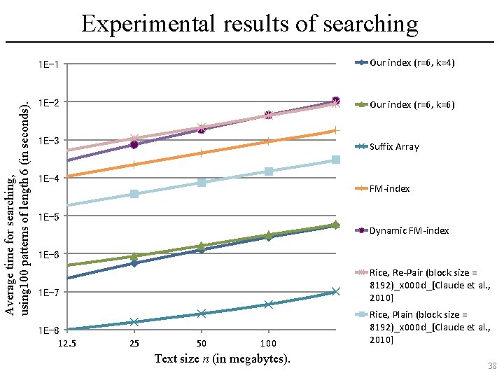
Average time for searching, using 100 patterns of length 6 (in seconds). Experimental results of searching 1 E-1 Our index (r=6, k=4) 1 E-2 Our index (r=6, k=6) 1 E-3 Suffix Array 1 E-4 FM-index 1 E-5 Dynamic FM-index 1 E-6 Rice, Re-Pair (block size = 8192)_x 000 d_[Claude et al. , 2010] 1 E-7 1 E-8 12. 5 25 50 100 Text size n (in megabytes). Rice, Plain (block size = 8192)_x 000 d_[Claude et al. , 2010] 38

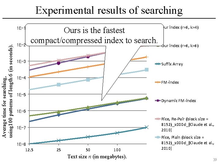
Experimental results of searching Average time for searching, using 100 patterns of length 6 (in seconds). 1 E-1 1 E-2 Ours is the fastest compact/compressed index to search. 1 E-3 Our index (r=6, k=4) Our index (r=6, k=6) Suffix Array 1 E-4 FM-index 1 E-5 Dynamic FM-index 1 E-6 Rice, Re-Pair (block size = 8192)_x 000 d_[Claude et al. , 2010] 1 E-7 1 E-8 12. 5 25 50 100 Text size n (in megabytes). Rice, Plain (block size = 8192)_x 000 d_[Claude et al. , 2010] 39

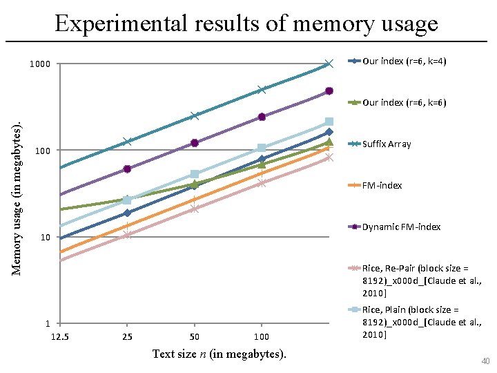
Experimental results of memory usage Our index (r=6, k=4) 1000 Memory usage (in megabytes). Our index (r=6, k=6) Suffix Array 100 FM-index Dynamic FM-index 10 Rice, Re-Pair (block size = 8192)_x 000 d_[Claude et al. , 2010] 1 12. 5 25 50 100 Text size n (in megabytes). Rice, Plain (block size = 8192)_x 000 d_[Claude et al. , 2010] 40

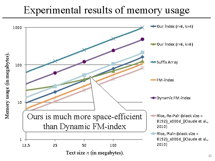
Experimental results of memory usage Our index (r=6, k=4) 1000 Memory usage (in megabytes). Our index (r=6, k=6) Suffix Array 100 FM-index Dynamic FM-index 10 Ours is much more space-efficient than Dynamic FM-index 1 12. 5 25 50 100 Text size n (in megabytes). Rice, Re-Pair (block size = 8192)_x 000 d_[Claude et al. , 2010] Rice, Plain (block size = 8192)_x 000 d_[Claude et al. , 2010] 41

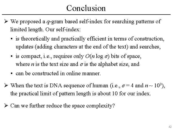
Conclusion Ø We proposed a q-gram based self-index for searching patterns of limited length. Our self-index: • is theoretically and practically efficient in terms of construction, updates (adding characters at the end of the text) and searches, • is compact, i. e. , requires only O(n log σ) bits of space, where n is the text size and σ is the alphabet size, and • can be constructed in online manner. Ø When the text is DNA sequence of human (i. e. , σ = 4 and n ~ 109), the practical limit of pattern length is about 10 for our index. Ø Can we further reduce the space complexity? 42