Semiclassical Physics of String Decay Jorge Russo University

Semiclassical Physics of String Decay Jorge Russo University of Barcelona - ICREA Based on R. Iengo and J. R. , “Handbook of string decay”, hepth/Jan 06 JHEP (2006) Santiago- February 2006

A highly excited quantum string state can be described in terms of a classical string. This state is unstable, and it can basically decay in two ways: 1) By splitting into two massive strings. 2) By emitting massless radiation. • Which is the dominant decay mode? • What is the lifetime? • How does it depend on the mass and on the “shape” of the string? • Does a string become more unstable for larger masses? • Is there any long-lived string state in the string spectrum? Computing the lifetime or decay rate of a given massive string state using string theory techniques is extremely complicated. It has been done only in few cases for specially simple states. Here we will derive simple rules to make a good estimate of the decay rate by splitting and massless radiation, and hence the lifetime of an arbitrary string state.

Decay Rate due to breaking 1. Open strings Probability for an open string to break: it is constant and proportional to g^2 [Dai, Polchinski (1989)] More precisely, we propose that the probability of breaking per unit time on a given point and at a given time once in a period is: T: period of oscillation of the string (so probability of breaking at any moment on a given point is T Po = g^2 ) In the “temporal” gauge, the period is essentially the mass:

Decay rate = Po times number of “points” times number of “instants”: This formula can be checked against the explicit quantum calculation of the decay rate for the open string with maximum angular momentum Jmax [Okada, Tsuchiya (1989)]. One finds in precise agreement with the above estimate.

Decay rates for open Jmax and closed Jmax.

2. Closed Strings In the absence of D-branes or fluxes, a closed string can only break into two outgoing closed strings. This means that the breaking is possible only if two points of the string meet. The possible configurations are: • The closed string is folded, with two sides in permanent contact. • The closed string becomes folded only at some instant of time. • The closed string has two points in permanent contact. • The closed string has two points which get in contact only at some instant of time. • The distance between any two points of the string is >>ls at all times. In this case the string is “unbreakable” and the decay rate into two massive string states is exponentially suppressed, Gamma=O(exp(-c. M 2))

Folded string The breaking can take place only if at a given time the two folds break at the same point, up to an uncertainty of order ls In particular, for the folded string with Jmax, Remarkably, it is constant independent of M.

A more precise comparison with the semiclassical estimate, requires separating the massless emission. The results are summarized in these figures:

Folded String wound n times The number of pairings between the 2 n folds of the string is ½ 2 n(2 n-1), so that

The string that becomes folded at an instant of time: The squashing closed string The process of breaking is possible only at the instant when the string is folded. Quantum mechanically, this represents a time interval of order ls Thus the rate is The last line applies to the squashing ellipse where L is proportional to M. This gives a lifetime

Lifetime for the squashing closed string in D = 10 and D = 4 computed from the one-string loop correction to the propagator.

Pulsating circular string This is a circular string which shrinks to a point once in a period. It can only break at the time when it is collapsed to a point. The decay rate can now be calculated just as in the squashing string case, but now taking into account that the two points where the breaking takes places are arbitrary, since all points get in contact. We get We can prove this remarkable identity analytically from the one-loop correction to the propagator (more on this later).

Strings with two points in permanent contact This is like the folded string, but now we do not have to multiply by the number of points of the string L/ls. We get Strings with finite number of contacts in one period This is obtained by adding a factor ls/T to the above result For these strings the decay rate due to breaking is very small and they are expected to decay primarily by massless radiation. An average string belong to this class.

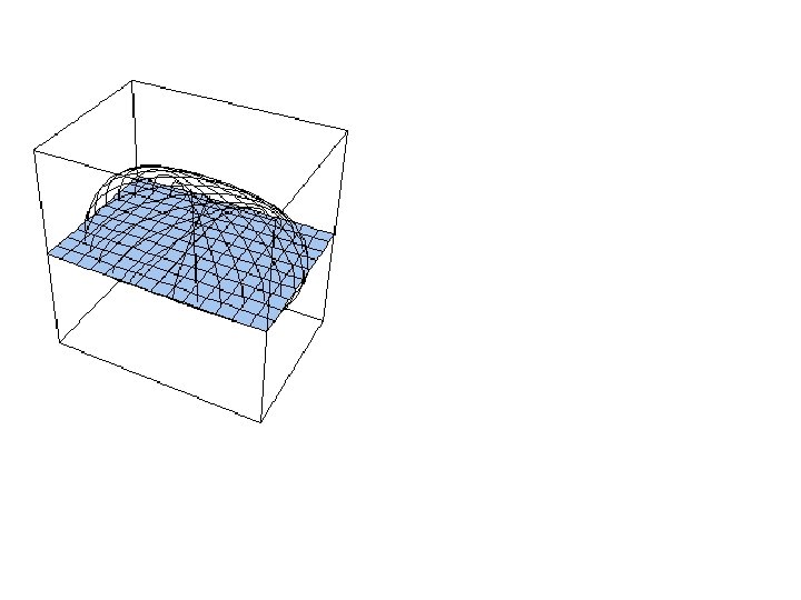
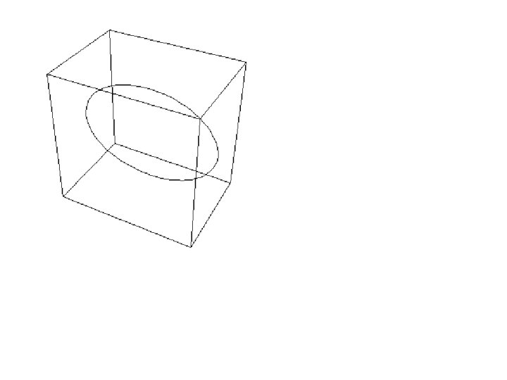
The squashing closed string For q generic, it describes an ellipse that rotates around one of its axes and simultaneously performs pulsations, with one of its radii becoming zero at t=n p. The solution interpolates between the folded string (q and the pulsating string (q =p/2) = 0)

Classical breaking The ellipse becomes folded at t = 0. We assume that the string breaks into two pieces at the points s=ap and s=2 p-ap. The outgoing strings, their masses and momenta can be determined by requiring continuity of X and the first time derivative of X at t = 0. Then we compute E, p, J for the strings I and II by integrating the canonical momenta associated with E, p, J in the intervals: I)s II ) s from 0 to s=ap and from s=2 p-ap to 2 p. from s=ap and from s=2 p-ap. We find • Independent of q. • Defines MI = f(MII)

Curve of classical splitting MI=f(MII) and maxima of G(MI, MII) for the squashing string

t = 0. 1 • The strings I and II rotate and pulsate. • They have two kinks which travel along the string. • At periodic times, they become folded. t = 0. 5

Evolution of the squashing closed string after splitting in the space ( y, z, t )

Splitting of Open string with Jmax In a generic situation, when an open string breaks, one kink on each of the outgoing strings is formed, which travels back and forth along the string [Iengo, J. R. , JHEP (2003)]

Quantum decay for the squashing closed string In type II superstring theory, the one-loop correction to the mass is given by • Compute fermion and boson correlators and sum over spin structures. • Next, one needs to integrate over z and tau : 1. One expands the holomorphic and antiholomorphic part of the integrand in powers of exp(i 2 p t) and exp(i 2 p z). 2. The integrals over the real parts of z and tau set the same power for each term in the holomorphic and antiholomorphic parts. 3. The integral over the imaginary part of z is a gaussian. 4. The integral over the imaginary part of tau is caried out by using the formula: The result is a function of x = sin q cos q. Therefore G(q=0) = G(q=p/2). This shows the remarkable fact that the quantum decay rate of the

The final result is a finite sum: It can be evaluated numerically. From this expression, we can see exactly what is decay rate due to radiation and what is the decay rate due to split into two massive strings:

Ratio GJmax/Gsquash as a function of M=sqrt[N]. Linear behavior, in agreement with the semiclassical prediction.

Decay rate due to massless emission • Contribution from four sectors NS-NS, R-NS, NS-R and R-R. • Computing massless decay rate for a generic quantum string state is very complicated. In particular, the covariant vertex operator is not known. • We have computed the quantum decay rate for every channel for the string Jmax and for the rotating ring. • There is one more case which can be computed: the average string state. • There is little chance that other cases (i. e. where the angular momentum is not near maximum or it is not the average) can ever be computed. Is there any way to estimate the string decay rate by massless emission? When the string is very massive, one can hope that the radiation can be described by the classical formula of gravitational radiation from a source Tmn(X). But this formula, in the most favorable cases, can only account for NS-NS radiation.

Rotating Ring: [Chialva, Iengo and J. R. ] • NS-NS emission is dominant. • R-NS and NS-R suppressed by 1/N , N=M 2. • R-R suppressed by 1/N 2. • NS-NS emission is accurately described by the classical formula: Identity between classical and quantum expressions up to terms of order 1/N. In general, the classical formula is expected to hold for graviton energies much less than the string mass =O(1/sqrt(a’)). If massless emission with higher energies is suppressed, then the classical formula can be used to compute the total decay rate by radiation emission In this regime w << O(1/sqrt(a’)) we expect that also NS-R, R-NS and R-R are also suppressed.

Classical formula: • Frame p = (w, -w, 0, . . . , 0) • Gauge X 0 = a’Mt • X+ , X- are light-cone coordinates. suppressed for high graviton energies w unless there is a saddle point. Two cases: 1. No saddle point (smooth strings): then the classical formula can be applied. Total radiation emission is convergent, and we get G = g 2 M 5 -D (very small in D>5!!!) 2. “Cusps” or “kinks” (discontinuities in derivatives of X). For D<=4 OK. (ex. Jmax) 3. [see Iengo and J. R, “Handbook of string decay” for more details; also Vilenkin, Damour]

Conclusions • By using simple rules we can estimate the decay rate into massive strings of any initial closed string configuration. These rules reproduce the quantum calculation in all specific cases that have been computed. • One can also have a reasonable control over the decay rate for massless emission, at least in D=4 or for smooth strings in any D. When the classical formula applies, the decay rate is G = g 2 M 5 -D. • In all cases, G string. = const. gs 2 M p, where p depends on the initial • We studied in detail the squashing string (containing the case of Jmax and circular pulsating strings). We find a perfect agreement between quantum decay rate and the semiclassical estimate. • A more general family of solutions can be written, which includes the squashing string and the rotating ring as particular cases. • Many possible applications, including Ad. S/CFT, cosmic strings, strings at LHC, etc.