Selforganizing maps SOMs and kmeans clustering Part 1

Self-organizing maps (SOMs) and k-means clustering: Part 1 Steven Feldstein The Pennsylvania State University Collaborators: Sukyoung Lee, Nat Johnson Trieste, Italy, October 21, 2013

Teleconnection Patterns • Atmospheric teleconnections are spatial patterns that link remote locations across the globe (Wallace and Gutzler 1981; Barnston and Livezey 1987) • Teleconnection patterns span a broad range of time scales, from just beyond the period of synoptic-scale variability, to interannual and interdecadal time scales.

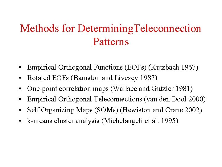
Methods for Determining. Teleconnection Patterns • • • Empirical Orthogonal Functions (EOFs) (Kutzbach 1967) Rotated EOFs (Barnston and Livezey 1987) One-point correlation maps (Wallace and Gutzler 1981) Empirical Orthogonal Teleconnections (van den Dool 2000) Self Organizing Maps (SOMs) (Hewiston and Crane 2002) k-means cluster analysis (Michelangeli et al. 1995)

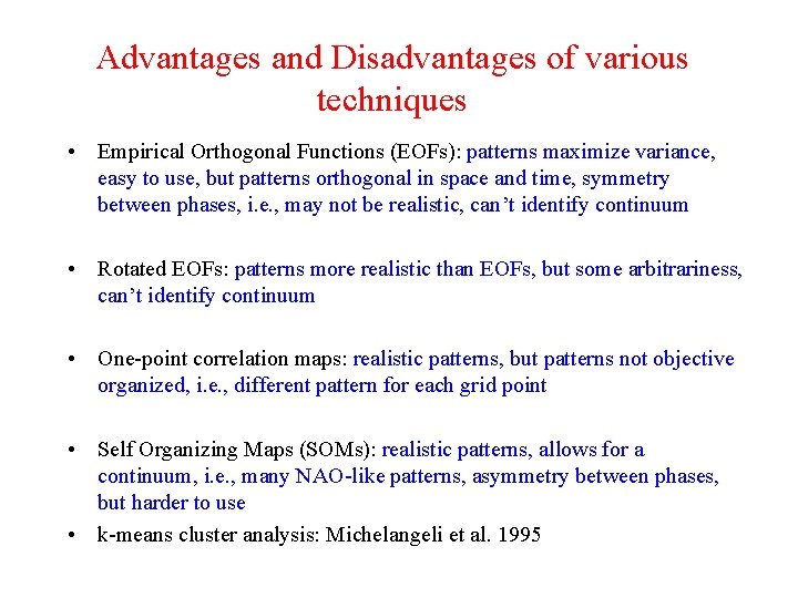
Advantages and Disadvantages of various techniques • Empirical Orthogonal Functions (EOFs): patterns maximize variance, easy to use, but patterns orthogonal in space and time, symmetry between phases, i. e. , may not be realistic, can’t identify continuum • Rotated EOFs: patterns more realistic than EOFs, but some arbitrariness, can’t identify continuum • One-point correlation maps: realistic patterns, but patterns not objective organized, i. e. , different pattern for each grid point • Self Organizing Maps (SOMs): realistic patterns, allows for a continuum, i. e. , many NAO-like patterns, asymmetry between phases, but harder to use • k-means cluster analysis: Michelangeli et al. 1995

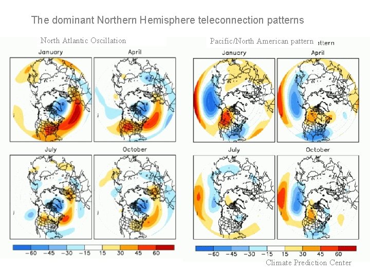
The dominant Northern Hemisphere teleconnection patterns North Atlantic Oscillation Pacific/North American pattern Climate Prediction Center

Aim of EOF, SOM analysis, and kmeans clustering • To reduce a large amount of data into a small number of representative patterns that capture a large fraction of the variability with spatial patterns that resemble the observed data

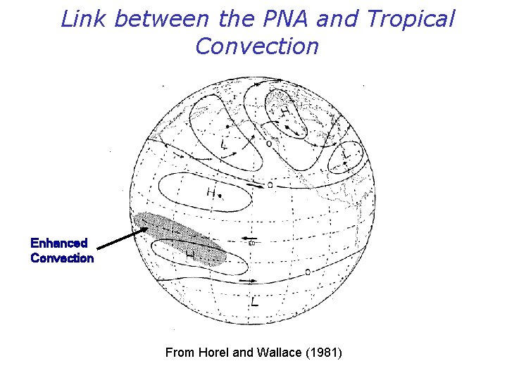
Link between the PNA and Tropical Convection Enhanced Convection From Horel and Wallace (1981)

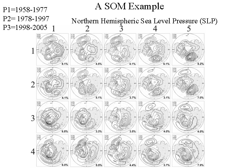
P 1=1958 -1977 P 2= 1978 -1997 P 3=1998 -2005 A SOM Example Northern Hemispheric Sea Level Pressure (SLP)

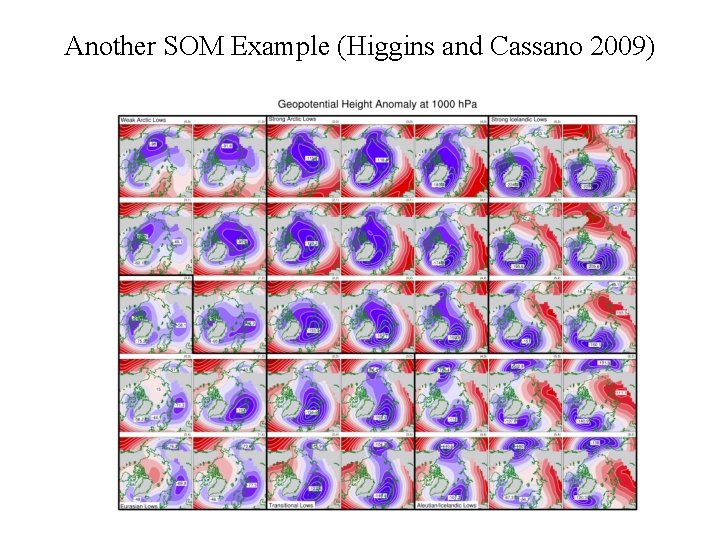
Another SOM Example (Higgins and Cassano 2009)

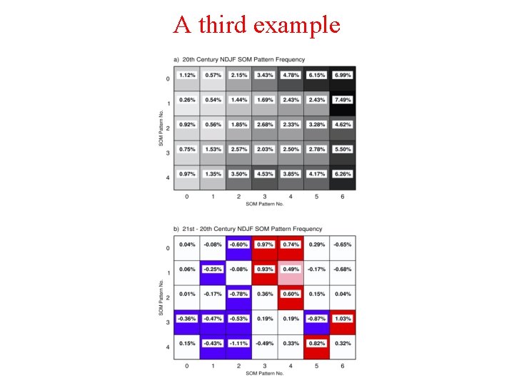
A third example

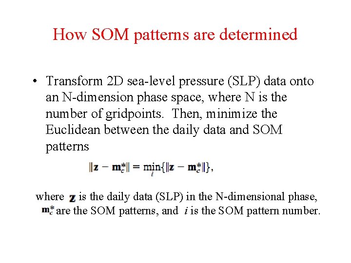
How SOM patterns are determined • Transform 2 D sea-level pressure (SLP) data onto an N-dimension phase space, where N is the number of gridpoints. Then, minimize the Euclidean between the daily data and SOM patterns where is the daily data (SLP) in the N-dimensional phase, are the SOM patterns, and i is the SOM pattern number.

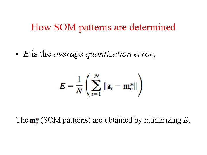
How SOM patterns are determined • E is the average quantization error, The (SOM patterns) are obtained by minimizing E.

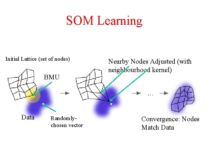
SOM Learning Initial Lattice (set of nodes) BMU Data Randomlychosen vector Nearby Nodes Adjusted (with neighbourhood kernel) Convergence: Nodes Match Data

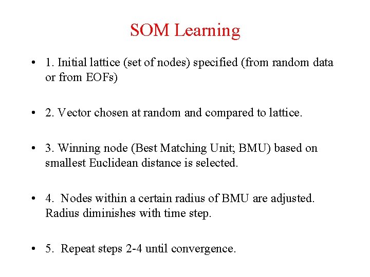
SOM Learning • 1. Initial lattice (set of nodes) specified (from random data or from EOFs) • 2. Vector chosen at random and compared to lattice. • 3. Winning node (Best Matching Unit; BMU) based on smallest Euclidean distance is selected. • 4. Nodes within a certain radius of BMU are adjusted. Radius diminishes with time step. • 5. Repeat steps 2 -4 until convergence.

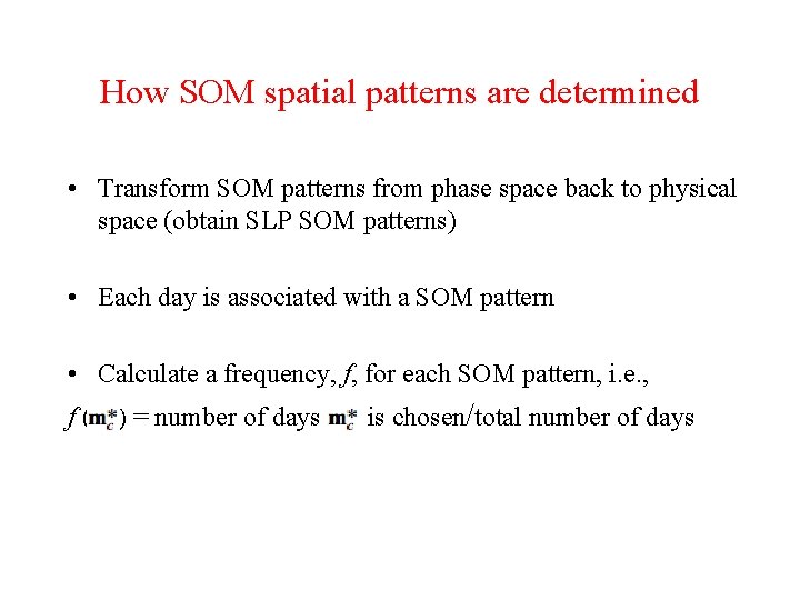
How SOM spatial patterns are determined • Transform SOM patterns from phase space back to physical space (obtain SLP SOM patterns) • Each day is associated with a SOM pattern • Calculate a frequency, f, for each SOM pattern, i. e. , f( ) = number of days is chosen/total number of days

SOMs are special! • Amongst cluster techniques, SOM analysis is unique in that it generates a 2 D grid with similar patterns nearby and dissimilar patterns widely separated.

Some Background on SOMs • SOM analysis is a type of Artificial Neural Network which generates a 2 -dimensional map (usually). This results in a low-dimensional view of the original high-dimension data, e. g. , reducing thousands of daily maps into a small number of maps. • SOMs were developed by Teuvo Kohonen of Finland.

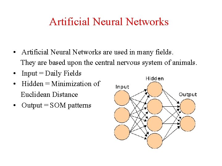
Artificial Neural Networks • Artificial Neural Networks are used in many fields. They are based upon the central nervous system of animals. • Input = Daily Fields • Hidden = Minimization of Euclidean Distance • Output = SOM patterns

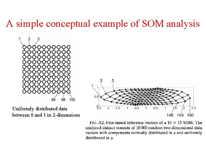
A simple conceptual example of SOM analysis Uniformly distributed data between 0 and 1 in 2 -dimensions

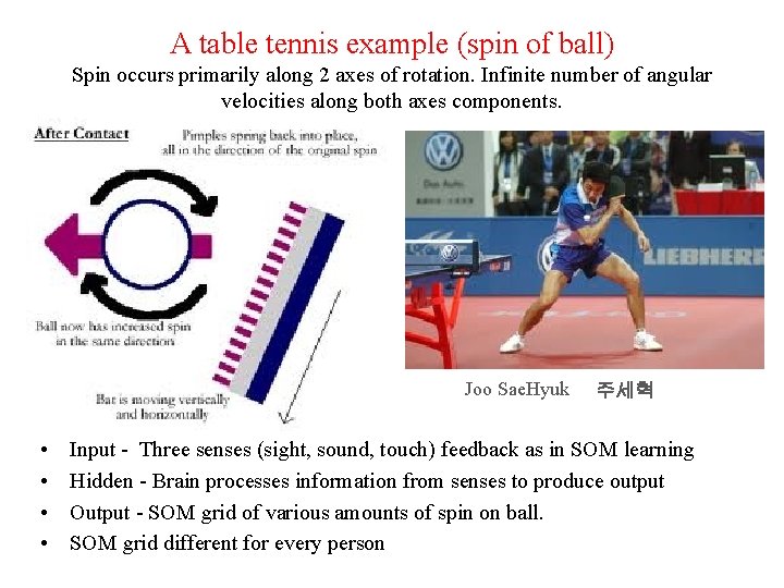
A table tennis example (spin of ball) Spin occurs primarily along 2 axes of rotation. Infinite number of angular velocities along both axes components. Joo Sae. Hyuk • • 주세혁 Input - Three senses (sight, sound, touch) feedback as in SOM learning Hidden - Brain processes information from senses to produce output Output - SOM grid of various amounts of spin on ball. SOM grid different for every person