Selfoptimizing control Simplementation of optimal operation Sigurd Skogestad

Self-optimizing control: Simplementation of optimal operation Sigurd Skogestad Department of Chemical Engineering Norwegian University of Science and Tecnology (NTNU) Trondheim, Norway ETH, Zürich, January 2009 (Based on presentation at 2008 Benelux control meeting) Effective Implementation of optimal operation using Off-Line Computations 1

Outline • Implementation of optimal operation • Paradigm 1: On-line optimizing control • Paradigm 2: "Self-optimizing" control schemes – Precomputed (off-line) solution • Control of optimal measurement combinations – Nullspace method – Exact local method • Link to optimal control / Explicit MPC • Current research issues 3

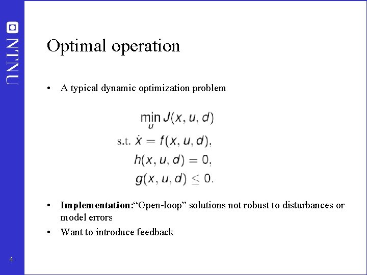
Optimal operation • A typical dynamic optimization problem • Implementation: “Open-loop” solutions not robust to disturbances or model errors • Want to introduce feedback 4

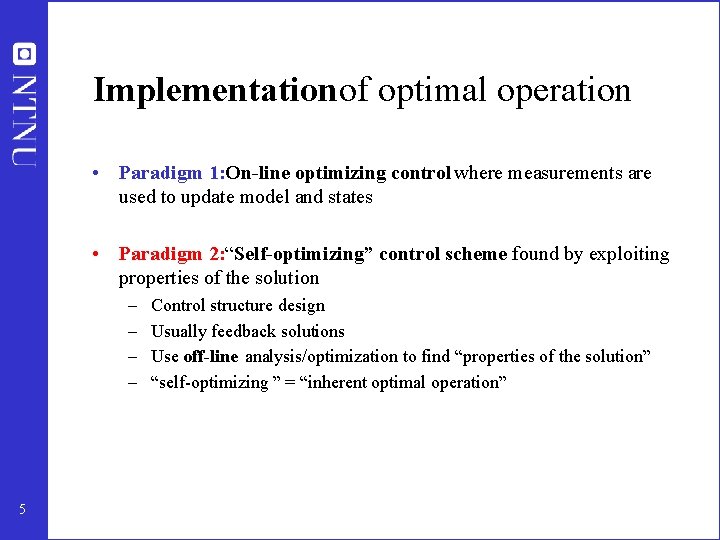
Implementation of optimal operation • Paradigm 1: On-line optimizing control where measurements are used to update model and states • Paradigm 2: “Self-optimizing” control scheme found by exploiting properties of the solution – – 5 Control structure design Usually feedback solutions Use off-line analysis/optimization to find “properties of the solution” “self-optimizing ” = “inherent optimal operation”

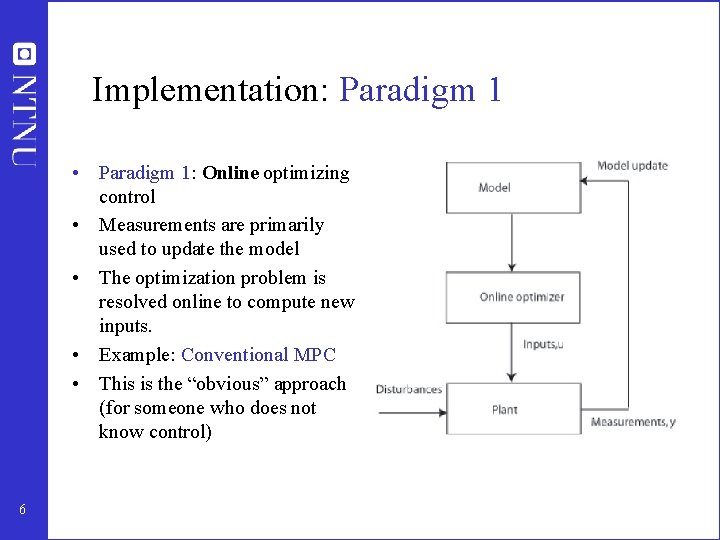
Implementation: Paradigm 1 • Paradigm 1: Online optimizing control • Measurements are primarily used to update the model • The optimization problem is resolved online to compute new inputs. • Example: Conventional MPC • This is the “obvious” approach (for someone who does not know control) 6

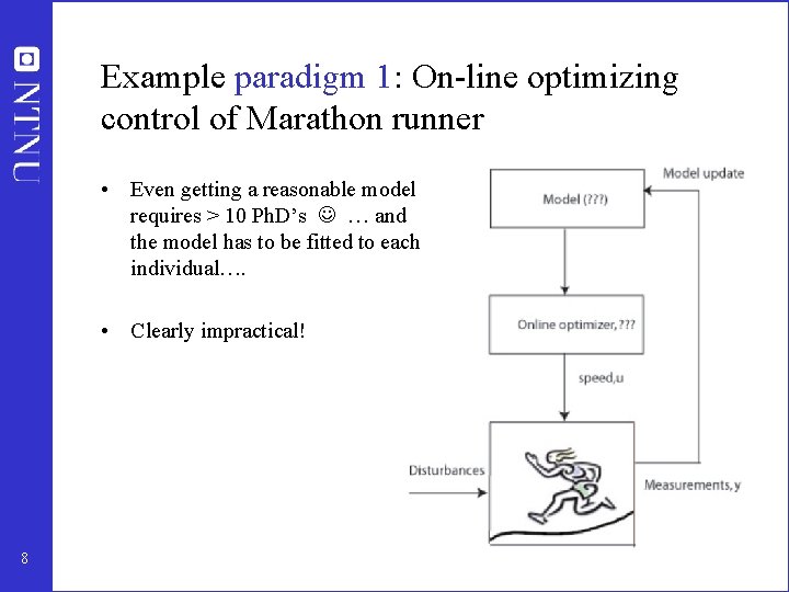
Example paradigm 1: On-line optimizing control of Marathon runner • Even getting a reasonable model requires > 10 Ph. D’s … and the model has to be fitted to each individual…. • Clearly impractical! 8

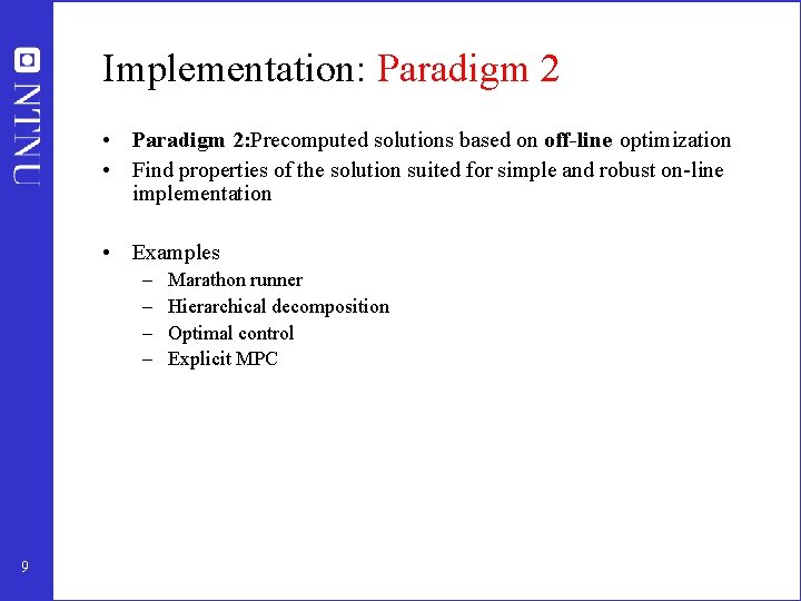
Implementation: Paradigm 2 • Paradigm 2: Precomputed solutions based on off-line optimization • Find properties of the solution suited for simple and robust on-line implementation • Examples – – 9 Marathon runner Hierarchical decomposition Optimal control Explicit MPC

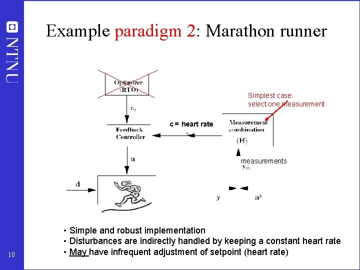
Example paradigm 2: Marathon runner Simplest case: select one measurement c = heart rate measurements 10 • Simple and robust implementation • Disturbances are indirectly handled by keeping a constant heart rate • May have infrequent adjustment of setpoint (heart rate)

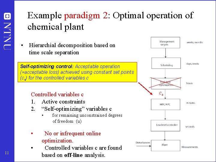
Example paradigm 2: Optimal operation of chemical plant • Hierarchial decomposition based on time scale separation Self-optimizing control: Acceptable operation (=acceptable loss) achieved using constant set points (cs) for the controlled variables c Controlled variables c 1. Active constraints 2. “Self-optimizing” variables c • • 11 • for remaining unconstrained degrees of freedom (u) No or infrequent online optimization. Controlled variables c are found based on off-line analysis. cs

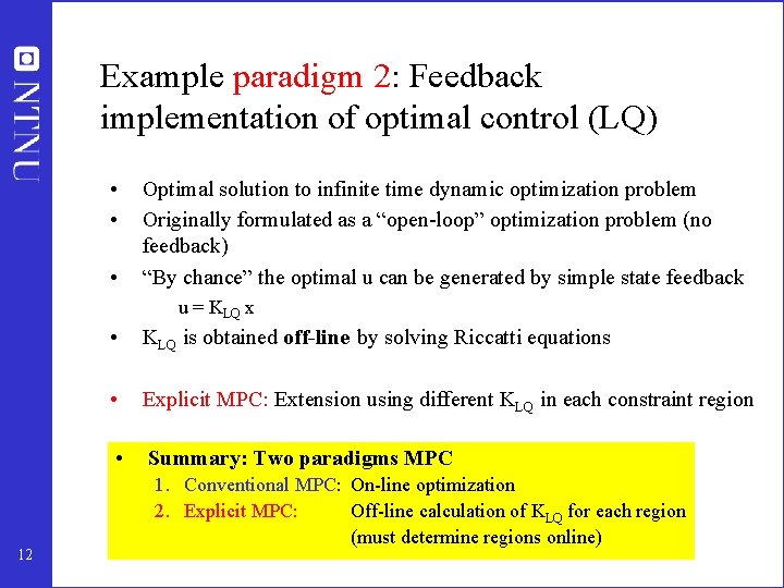
Example paradigm 2: Feedback implementation of optimal control (LQ) • • • Optimal solution to infinite time dynamic optimization problem Originally formulated as a “open-loop” optimization problem (no feedback) “By chance” the optimal u can be generated by simple state feedback u = KLQ x 12 • KLQ is obtained off-line by solving Riccatti equations • Explicit MPC: Extension using different KLQ in each constraint region • Summary: Two paradigms MPC 1. Conventional MPC: On-line optimization 2. Explicit MPC: Off-line calculation of KLQ for each region (must determine regions online)

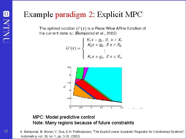
Example paradigm 2: Explicit MPC: Model predictive control Note: Many regions because of future constraints 13 A. Bemporad, M. Morari, V. Dua, E. N. Pistikopoulos, ”The Explicit Linear Quadratic Regulator for Constrained Systems”, Automatica, vol. 38, no. 1, pp. 3 -20 (2002).

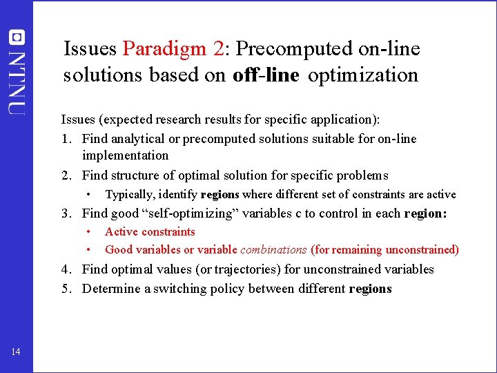
Issues Paradigm 2: Precomputed on-line solutions based on off-line optimization Issues (expected research results for specific application): 1. Find analytical or precomputed solutions suitable for on-line implementation 2. Find structure of optimal solution for specific problems • Typically, identify regions where different set of constraints are active 3. Find good “self-optimizing” variables c to control in each region: • • Active constraints Good variables or variable combinations (for remaining unconstrained) 4. Find optimal values (or trajectories) for unconstrained variables 5. Determine a switching policy between different regions 14

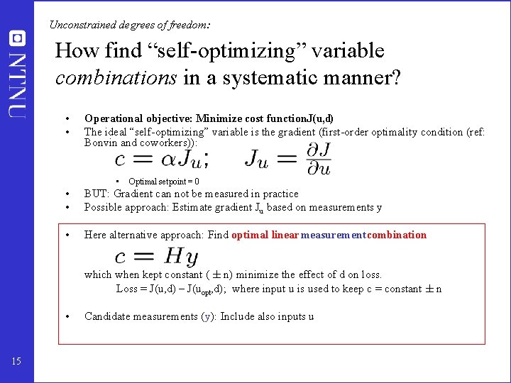
Unconstrained degrees of freedom: How find “self-optimizing” variable combinations in a systematic manner? • • Operational objective: Minimize cost function. J(u, d) The ideal “self-optimizing” variable is the gradient (first-order optimality condition (ref: Bonvin and coworkers)): • Optimal setpoint = 0 • • BUT: Gradient can not be measured in practice Possible approach: Estimate gradient Ju based on measurements y • Here alternative approach: Find optimal linear measurementcombination which when kept constant ( § n) minimize the effect of d on loss. Loss = J(u, d) – J(uopt, d); where input u is used to keep c = constant § n • 15 Candidate measurements (y): Include also inputs u

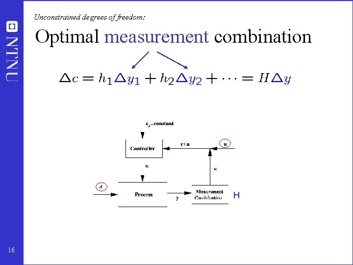
Unconstrained degrees of freedom: Optimal measurement combination H 16

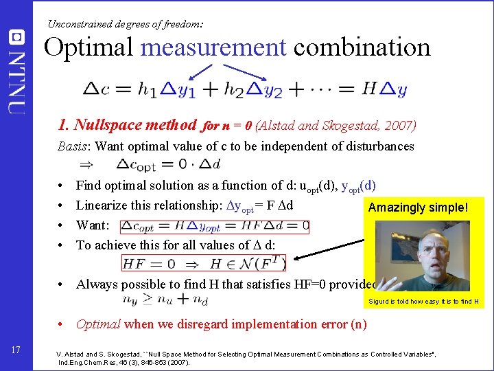
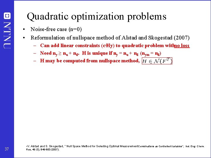
Unconstrained degrees of freedom: Optimal measurement combination 1. Nullspace method for n = 0 (Alstad and Skogestad, 2007) Basis: Want optimal value of c to be independent of disturbances • • Find optimal solution as a function of d: uopt(d), yopt(d) Linearize this relationship: yopt = F d Amazingly simple! Want: To achieve this for all values of d: • Always possible to find H that satisfies HF=0 provided Sigurd is told how easy it is to find H • Optimal when we disregard implementation error (n) 17 V. Alstad and S. Skogestad, ``Null Space Method for Selecting Optimal Measurement Combinations as Controlled Variables'', Ind. Eng. Chem. Res, 46 (3), 846 -853 (2007).

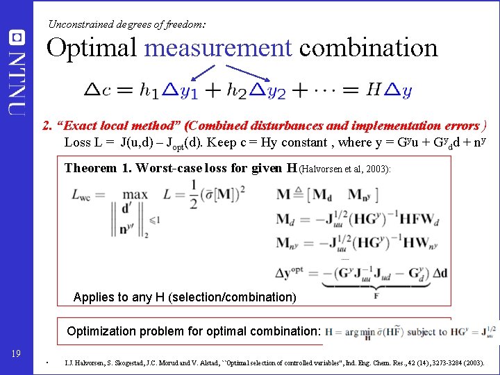
Unconstrained degrees of freedom: Optimal measurement combination 2. “Exact local method” (Combined disturbances and implementation errors ) Loss L = J(u, d) – Jopt(d). Keep c = Hy constant , where y = Gyu + Gydd + ny Theorem 1. Worst-case loss for given H (Halvorsen et al, 2003): Applies to any H (selection/combination) Optimization problem for optimal combination: 19 • I. J. Halvorsen, S. Skogestad, J. C. Morud and V. Alstad, ``Optimal selection of controlled variables'', Ind. Eng. Chem. Res. , 42 (14), 3273 -3284 (2003).

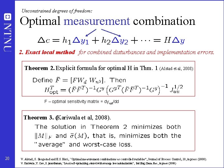
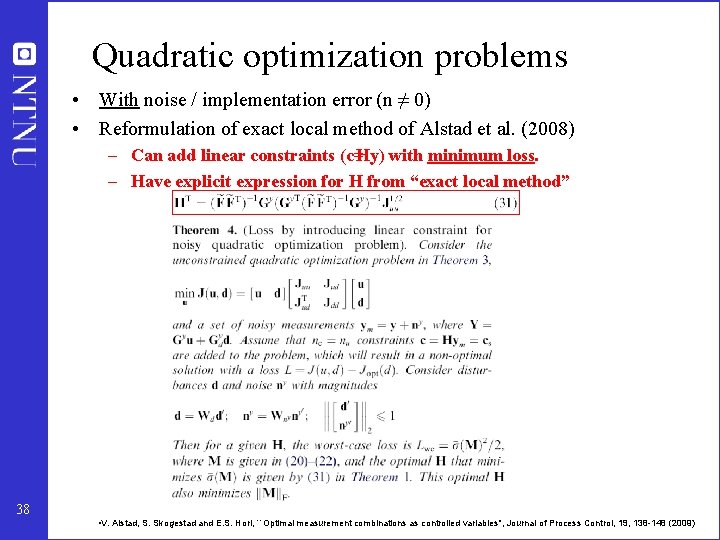
Unconstrained degrees of freedom: Optimal measurement combination 2. Exact local method for combined disturbances and implementation errors. Theorem 2. Explicit formula for optimal H in Thm. 1 (Alstad et al, 2008): F – optimal sensitivity matrix = dyopt/dd Theorem 3. (Kariwala et al, 2008). 20 V. Alstad, S. Skogestad and E. S. Hori, ``Optimal measurement combinations as controlled variables'', Journal of Process Control, 18, in press (2008). V. Kariwala, Y. Cao, S. jarardhanan, “Local self-optimizing control with average loss minimization”, Ind. Eng. Chem. Res. , in press (2008)

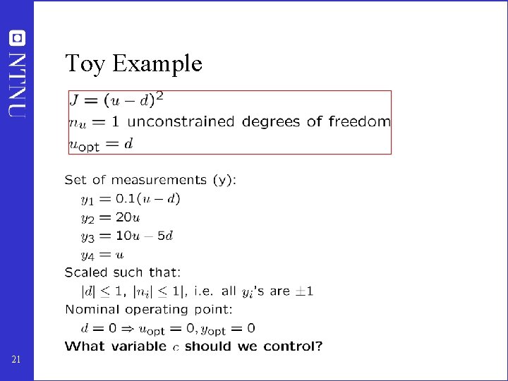
Toy Example 21

Toy Example: Single measurements Constant input, c = y 4 = u 22 Want loss < 0. 1: Consider variable combinations

Toy Example: Measurement combinations 23

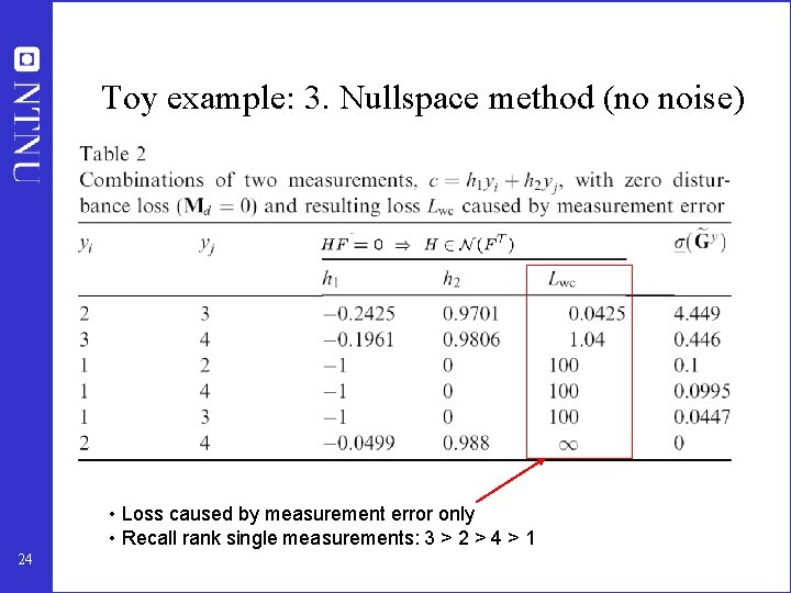
Toy example: 3. Nullspace method (no noise) • Loss caused by measurement error only • Recall rank single measurements: 3 > 2 > 4 > 1 24

4. Exact local method (with noise) 25

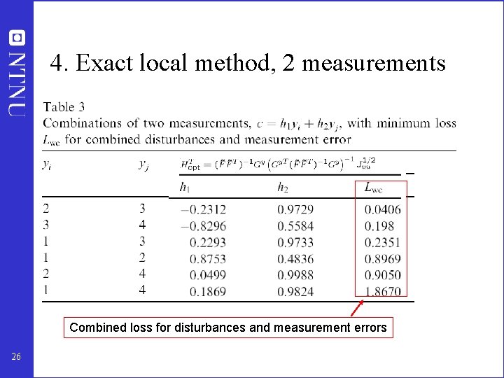
4. Exact local method, 2 measurements Combined loss for disturbances and measurement errors 26

4. Exact local method, all 4 measurements 27

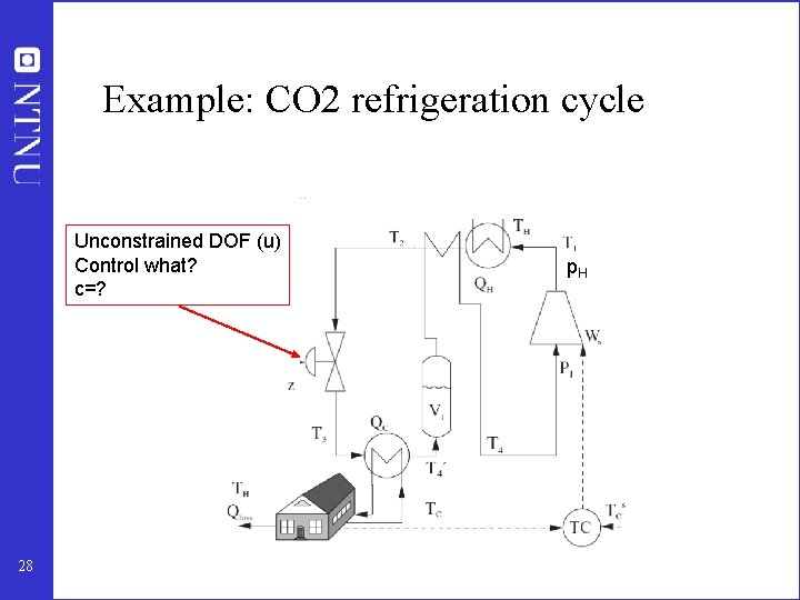
Example: CO 2 refrigeration cycle Unconstrained DOF (u) Control what? c=? 28 p. H

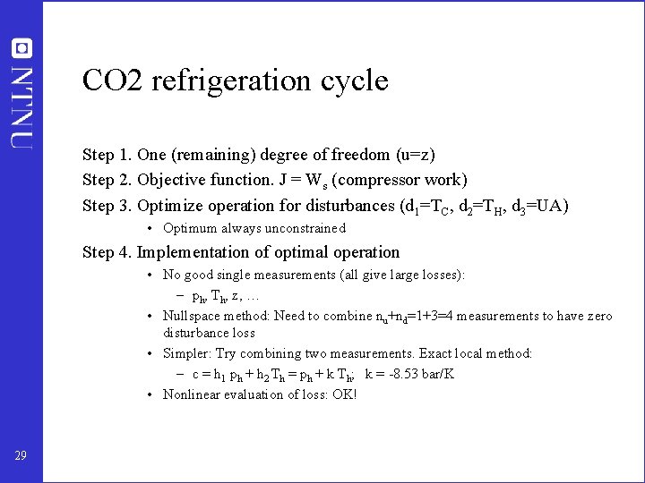
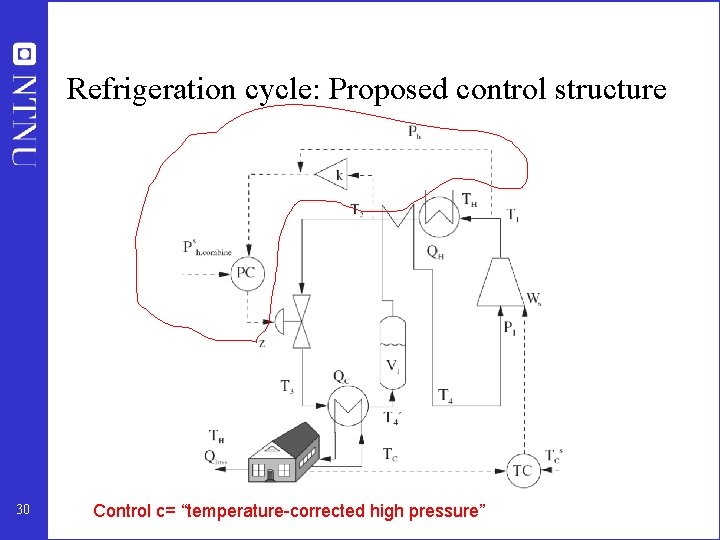
CO 2 refrigeration cycle Step 1. One (remaining) degree of freedom (u=z) Step 2. Objective function. J = Ws (compressor work) Step 3. Optimize operation for disturbances (d 1=TC, d 2=TH, d 3=UA) • Optimum always unconstrained Step 4. Implementation of optimal operation • No good single measurements (all give large losses): – ph, Th, z, … • Nullspace method: Need to combine nu+nd=1+3=4 measurements to have zero disturbance loss • Simpler: Try combining two measurements. Exact local method: – c = h 1 ph + h 2 Th = ph + k Th; k = -8. 53 bar/K • Nonlinear evaluation of loss: OK! 29

Refrigeration cycle: Proposed control structure 30 Control c= “temperature-corrected high pressure”

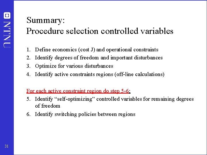
Summary: Procedure selection controlled variables 1. 2. 3. 4. Define economics (cost J) and operational constraints Identify degrees of freedom and important disturbances Optimize for various disturbances Identify active constraints regions (off-line calculations) For each active constraint region do step 5 -6: 5. Identify “self-optimizing” controlled variables for remaining degrees of freedom 6. Identify switching policies between regions 31

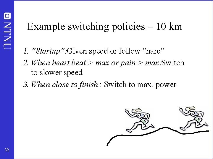
Example switching policies – 10 km 1. ”Startup”: Given speed or follow ”hare” 2. When heart beat > max or pain > max: Switch to slower speed 3. When close to finish : Switch to max. power 32

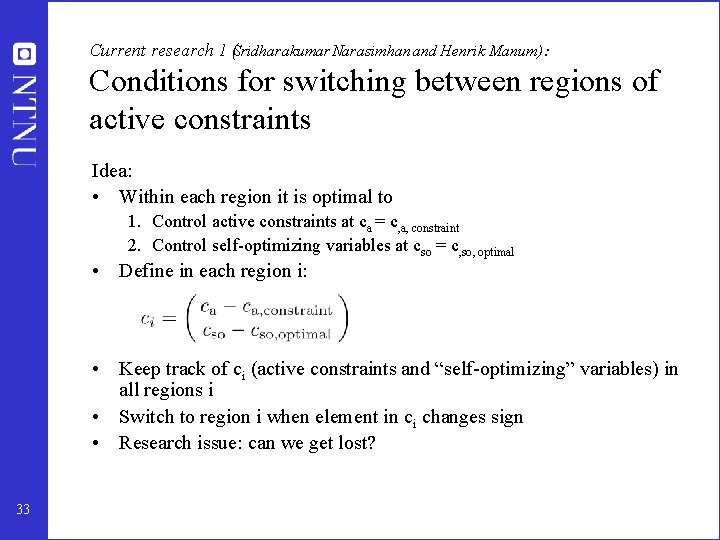
Current research 1 (Sridharakumar Narasimhan and Henrik Manum): Conditions for switching between regions of active constraints Idea: • Within each region it is optimal to 1. Control active constraints at ca = c, a, constraint 2. Control self-optimizing variables at cso = c, so, optimal • Define in each region i: • Keep track of ci (active constraints and “self-optimizing” variables) in all regions i • Switch to region i when element in ci changes sign • Research issue: can we get lost? 33

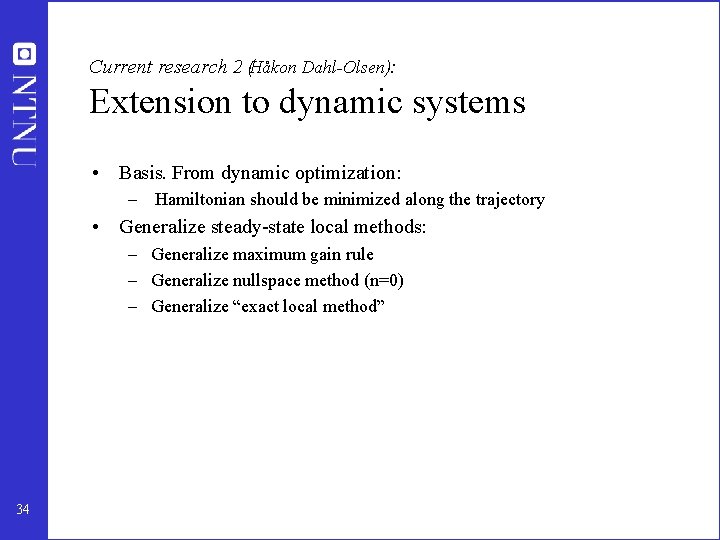
Current research 2 (Håkon Dahl-Olsen): Extension to dynamic systems • Basis. From dynamic optimization: – Hamiltonian should be minimized along the trajectory • Generalize steady-state local methods: – Generalize maximum gain rule – Generalize nullspace method (n=0) – Generalize “exact local method” 34

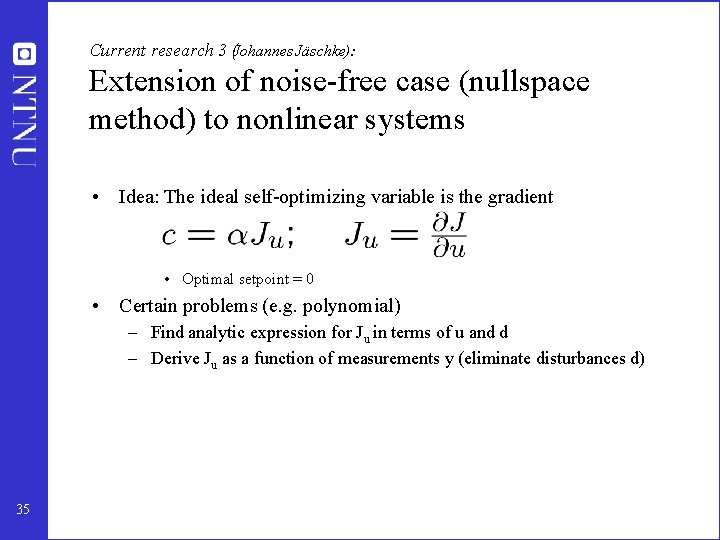
Current research 3 (Johannes Jäschke): Extension of noise-free case (nullspace method) to nonlinear systems • Idea: The ideal self-optimizing variable is the gradient • Optimal setpoint = 0 • Certain problems (e. g. polynomial) – Find analytic expression for Ju in terms of u and d – Derive Ju as a function of measurements y (eliminate disturbances d) 35

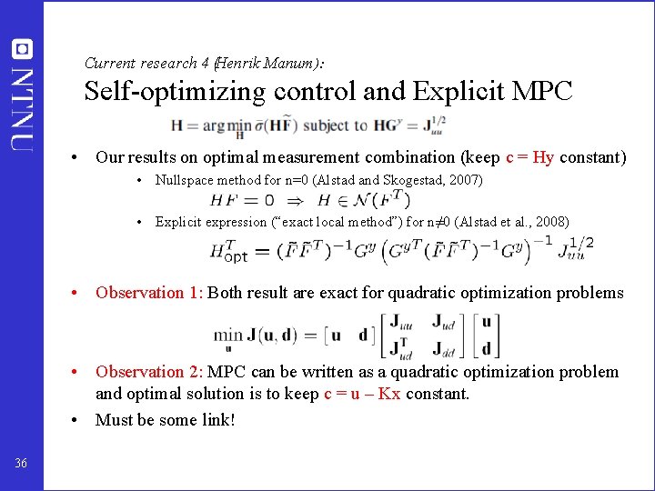
Current research 4 (Henrik Manum ): Self-optimizing control and Explicit MPC • Our results on optimal measurement combination (keep c = Hy constant) • Nullspace method for n=0 (Alstad and Skogestad, 2007) • Explicit expression (“exact local method”) for n≠ 0 (Alstad et al. , 2008) • Observation 1: Both result are exact for quadratic optimization problems • Observation 2: MPC can be written as a quadratic optimization problem and optimal solution is to keep c = u – Kx constant. • Must be some link! 36

Quadratic optimization problems • Noise-free case (n=0) • Reformulation of nullspace method of Alstad and Skogestad (2007) – Can add linear constraints (c=Hy) to quadratic problem withno loss – Need ny ≥ nu + nd. H is unique if ny = nu + nd (nym = nd) – H may be computed from nullspace method, 37 • V. Alstad and S. Skogestad, ``Null Space Method for Selecting Optimal Measurement Combinations as Controlled Variables'', Ind. Eng. Chem. Res, 46 (3), 846 -853 (2007).

Quadratic optimization problems • With noise / implementation error (n ≠ 0) • Reformulation of exact local method of Alstad et al. (2008) – Can add linear constraints (c=Hy) with minimum loss. – Have explicit expression for H from “exact local method” 38 • V. Alstad, S. Skogestad and E. S. Hori, ``Optimal measurement combinations as controlled variables'', Journal of Process Control, 19, 138 -148 (2009)

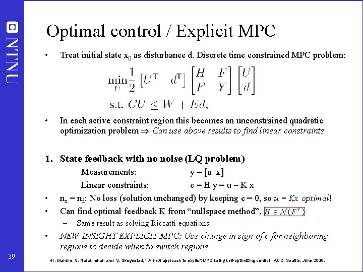
Optimal control / Explicit MPC • Treat initial state x 0 as disturbance d. Discrete time constrained MPC problem: • In each active constraint region this becomes an unconstrained quadratic optimization problem ) Can use above results to find linear constraints 1. State feedback with no noise (LQ problem) • • Measurements: y = [u x] Linear constraints: c=Hy=u–Kx nx = nd: No loss (solution unchanged) by keeping c = 0, so u = Kx optimal! Can find optimal feedback K from “nullspace method”, – • 39 Same result as solving Riccatti equations NEW INSIGHT EXPLICIT MPC: Use change in sign of c for neighboring regions to decide when to switch regions • H. Manum, S. Narasimhan and S. Skogestad, ``A new approach to explicit MPC using self-optimizing control”, ACC, Seattle, June 2008.

Explicit MPC. State feedback. Second-order system Phase plane trajectory 40 time [s]

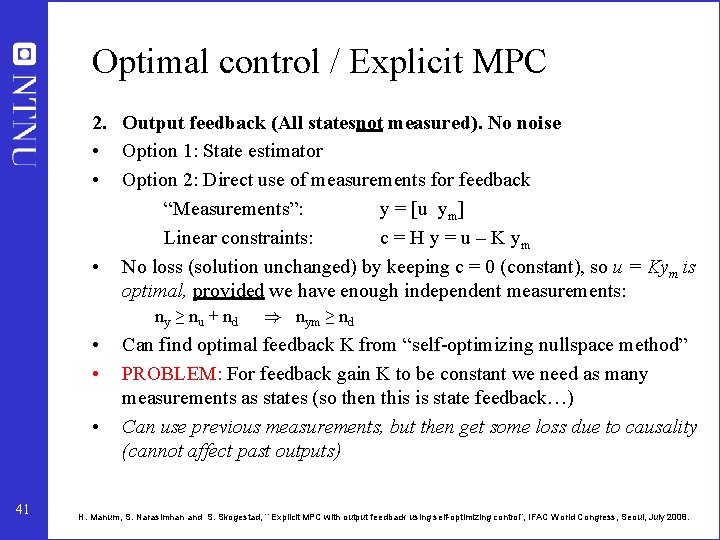
Optimal control / Explicit MPC 2. Output feedback (All statesnot measured). No noise • Option 1: State estimator • Option 2: Direct use of measurements for feedback “Measurements”: y = [u ym] Linear constraints: c = H y = u – K ym • No loss (solution unchanged) by keeping c = 0 (constant), so u = Kym is optimal, provided we have enough independent measurements: ny ≥ nu + nd • • • 41 ) nym ≥ nd Can find optimal feedback K from “self-optimizing nullspace method” PROBLEM: For feedback gain K to be constant we need as many measurements as states (so then this is state feedback…) Can use previous measurements, but then get some loss due to causality (cannot affect past outputs) H. Manum, S. Narasimhan and S. Skogestad, ``Explicit MPC with output feedback using self-optimizing control”, IFAC World Congress, Seoul, July 2008.

Explicit MPC. Output feedback Second-order system State feedback 42 time [s]

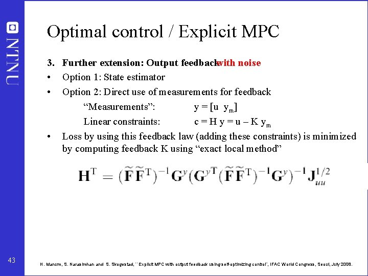
Optimal control / Explicit MPC 3. Further extension: Output feedbackwith noise • Option 1: State estimator • Option 2: Direct use of measurements for feedback “Measurements”: y = [u ym] Linear constraints: c = H y = u – K ym • Loss by using this feedback law (adding these constraints) is minimized by computing feedback K using “exact local method” 43 H. Manum, S. Narasimhan and S. Skogestad, ``Explicit MPC with output feedback using self-optimizing control”, IFAC World Congress, Seoul, July 2008.

Conclusion • Simple control policies are always preferred in practice (if they exist and can be found) • Paradigm 2: Use off-line optimization and analysis to find simple near -optimal control policies suitable for on-line implementation • Current research: Several interesting extensions – Optimal region switching – Dynamic optimization – Explicit MPC • 44 Acknowledgements – Sridharakumar Narasimhan – Henrik Manum – Håkon Dahl-Olsen – Vinay Kariwala