Selection on unobservables Using natural experiments to identify

Selection on unobservables Using natural experiments to identify causal effects

Selection on unobservables • Recall the identifying assumptions when estimates causal effect using conditioning strategies – Independence: (Y 0, Y 1) || D, X • Condition on exogenous covariates that close all open backdoor paths – Do not condition on colliders – Use methods like propensity score matching and condition on p(X), or regression • What if treatment assignment to units based on some unobserved variable, u, which is correlated with the outcome? – Conditioning strategies are invalid – Selection on unobservables methods may work • Angrist and Lavy (1999): “Using Maimonedes’ Rule to Estimate the Effect of Class Size on Scholastic Achievement”, Quarterly Journal of Economics

Maimonedes Rule “Causal effects of class size on pupil achievement have proved very difficult to measure. Even though the level of educational inputs differs substantially both between and within schools, these differences are often associated with factors such as remedial training or students’ socioeconomic background … The great twelfth century Rabbinic scholar, Maimonides, interprets the Talmud’s discussion of class size as follows: “Twenty-five children may be put in charge of one teacher. If the number in the class exceeds twenty-five but is not more than forty, two teachers must be appointed. ’ … The importance of Maimonides’ rule for our purposes is that since 1969, it has been used to determine the division of enrollment cohorts into classes in Israeli public schools. ” (Angrist and Lavy 1999).
 are interested in the causal")
Natural experiments: Example 1 • Angrist and Lavy (1999) are interested in the causal effect of class size (D) on education outcomes (Y) • Data: 86 paired Israeli schools matched on covariate, x (share of disadvantaged children) – They were matched on observable covariate x – but are treatment group students equivalent to control on both x and u, not just x? • Treatment: Small class size is the treatment – Treatment: 41 -50 students in 5 th grade (D=1) – Control: 31 -40 students in 5 th grade (D=0)

Exogenous variation in class size • Class size in most places and most times is strongly associated with unobservable determinants of educational performance – Poverty, affluence, enthusiasm or skepticism about the value of education, special needs of students for remedial or advanced instruction, obscure and barely intelligible obsessions of bureaucracies – Each of these determines class size and clouds the actual effect of class size on academic performance because each is also correlated with academic performance itself • However, if adherence to Maimonides’ rule is perfectly rigid, then what separates School A with a single class of size 40 from School B with two classes whose average size is 20. 5? – the enrollment of a single student

Exogenous variation in class size Maimonides’ rule has the largest impact on a school with about 40 students in a grade cohort are With cohorts of size 40, 80 and 120 students, the steps down in average class size required by Maimonides’ rule when an additional student enrolls (respectively) from 40 to 20. 5 (41/2), 40 to 27 (81/3) and 40 to 30. 25 (121/3) Schools also use the percent disadvantaged students in a school “to allocate supplementary hours of instruction and other school resources”, so Angrist and Lavy created 86 matched pairs of schools using this covariate, x Upper left panel: balanced on x; top right shows Maimonides Rule working; bottom left and right: math and verbal test scores were higher where class sizes tended to be smaller
-Natural experiments • • Angrist and Lavy (1999) are interested in the causal effect")
(Un)-Natural experiments • • Angrist and Lavy (1999) are interested in the causal effect of class size on academic performance, and while they can match on observables, it is widely known that selection on unobservables is a more apt description of the problem They solve this problem by exploiting Maimonides’ Rule – Maimonides’ Rule cuts classes in half when they reach a prescribed point – The key is that the decision to create classes of different sizes is based on an arbitrary cutoff which is unrelated to unobservable determinants of D or Y • They call it a “natural experiment” but what does that mean? – An attempt to find in the world some rare circumstance such that a consequential treatment was handed to some people and denied to others haphazard reasons – Caveat: “The word `natural’ has various connotations, but a `natural experiment’ is a `wild experiment’ not a `wholesome experiment’, nature in the way that a tiger is natural, not in the way that oatmeal is natural” (Rosenbaum 2005, Design of Observational Studies) • Haphazard variation in treatment is not like variation in a randomized experiment – Randomization: “We definitely know that the probability of treatment for the large class size and the small class size units was equal by the way treatments were assigned”, versus – Natural experiment: “It does seem reasonably plausible that the probability of treatment for the kids in the small class sizes and the kids in the large class sizes is fairly close”.

Treatment selection and naiveté • Naïve matching – “People who look comparable are comparable”. NO • Matching/subclassification/regression can create matched sample who look similar on x • Matching, etc. cannot created a matched sample who are similar on u (unobservables), though • Definition of naiveté: a person who believes something because it’s convenient to believe it
 Dr. John Snow was: • A")
Story of the Broad Street Pump (ex. 2) Dr. John Snow was: • A practicing physician • An anesthesiologist • Studied “poisons / morbid matters • Father of epidemiology • • Provided early evidence that cholera was waterborne disease He lived from 1813 1858

Cholera science in 1800 s • Go back in time and forget that germs cause disease – Microscopes were available but their resolution was poor – Most human pathogens can’t be seen – Isolating these microorganisms wouldn’t occur for half a century • The “infection theory” was the minority view; main explanation was “miasmas” – Minute, inanimate poison particles in the air

Background • Cholera arrives in Europe in the early 1800 s and exhibits “epidemic waves” – Attacked victims suddenly – Usually fatal – Symptoms were vomiting and acute diarrhea • Snow observed the clinical course of the disease and made the following conjecture: – the active agent was a living organism that entered the body, got into the alimentary canal with food or drink, multiplied in the body, and generated some poison that caused the body to expel water – The organism passed out of the body with these evacuations, entered the water supply, and infected new victims – The process would repeat itself, growing rapidly through the common water supply, causing an epidemic • There were three main epidemics in London – 1831 -1832 – 1848 -1849 (~15, 000 deaths) – 1853 -1854 (~30, 000 deaths)

Background • Snow is an early advocate for the “infection theory” – cholera is being spread person-to-person through an unknown mechanism • His early evidence for this “infection theory” was based on years’ worth of observations which included: – Cholera transmission followed human commerce – A sailor on a ship from a cholera-free country who arrived at a cholera-stricken port would only get the disease after landing or taking on supplies – Cholera hit poor communities the worst, who lived in the most crowded housing with the worst hygiene • These facts are consistent with the infection theory, but were harder to reconcile with the miasma theory

More observational evidence supporting Snow’s infection theory • Snow identifies Patient Zero: the first case of an early epidemic: – “a seaman named John Harnold, who had arrived by the Elbe steamer from Hamburg, where the disease was prevailing • The second case is Harnold’s roommate

And more evidence from later epidemics • Snow studied two apartment buildings – The 1 st was heavily hit with cholera, but the 2 nd wasn’t – He found the water supply in the 1 st building was contaminated by runoff from privies but the water supply in the 2 nd was much cleaner • Earlier water supply studies – In the London of the 1800 s, there were many different water companies serving different areas of the city – Some were served by more than one company – Several took their water from the Thames, which was heavily polluted by sewage – The service areas of such companies had much higher rates of cholera – The Chelsea water company was an exception, but it had an exceptionally good filtration system

Broad Street Water Pump • 1849: – Lambeth water company moved the intake point upstream along the Thames, above the main sewage discharge points • Pure water – Southwark and Vauxhall water company left their intake point downstream from where the sewage discharged • Infected water • Comparisons of data on cholera deaths from the 185354 showed that the epidemic hit harder in the Southwark and Vauxhall service areas (infected water supply) and largely spared the Lambeth areas (pure water)

Snow’s Table IX Number of houses Deaths from cholera Deaths per 10, 000 houses Southwark and Vauxhall 40, 046 1, 263 315 Lambeth 26, 107 98 37 Rest of London 256, 423 1, 422 59 Snow concluded that if the Southwark and Vauxhall company had moved their intake point as Lambeth did, about 1, 000 lives would have been saved. Counterfactual inference, quasi-randomized treatment assignment to control for confounding variables

So what about u?


Snow’s Table IX Number of houses Deaths from cholera Deaths per 10, 000 houses Southwark and Vauxhall 40, 046 1, 263 315 Lambeth 26, 107 98 37 Rest of London 256, 423 1, 422 59 David Freedman (1991)’s “Statistical Models and Shoe Leather”: “As a piece of statistical technology, [Snow’s Table IX] is by no means remarkable. But the story it tells is very persuasive. The force of the argument results from the clarity of the prior reasoning, the bringing together of many different lines of evidence, and the amount of shoe leather Snow was willing to use to get the data. ” “Snow did some brilliant detective work on nonexperimental data. What is impressive is not the statistical technique but the handling of the scientific issues. He made steady progress from shrewd observation through case studies to analyze ecological data. In the end, he found analyzed a natural experiment. “He also made his share of mistakes: For example, based on rather flimsy analogies, he concluded that plague and yellow fever were also propagated through the water. ”
 • Kanarek, et. al. (1980), American Journal of Epidemiology (leading")
Example 3 (bad example) • Kanarek, et. al. (1980), American Journal of Epidemiology (leading journal in the field) – Big finding: asbestos fibers in drinking water caused lung cancer – 722 census tracts in San Francisco Bay Area – Large variations in fiber concentrations from one tract to another (by factors of 10 or more) – Examined cancer rates at 35 sites for blacks and whites, men and women – Controlled for age, sex and race, and used loglinear regression to control for other covariates – Causation was inferred based on whether a coefficient in the model was statistically significant after controlling for covariates
 do not discuss their stochastic")
Asbestos and lung cancer • Kanarek et al (1980) do not discuss their stochastic assumptions – Their model assumes independence of treatment assignment conditional covariates – Regression language: they assume conditional independence – that the error term is i. i. d. given covariates and treatment is conditionally exogenous – without justification • “Theoretical construction of the probability of developing cancer by a certain time yields a function of the log form” (1980, p. 62) • But this model of cancer causation is open to serious objections (Freedman and Navidi 1989) • Findings – First, they confuse “statistical significance” for “economic significance”: • For lung cancer in white males, the asbestos fiber coefficient was highly significant ( p<0. 001), so the “effect” was described as “strong” • But in reality, their model actually only predicts a risk multiplier of 1. 05 for 100 -fold increase in fiber concentrations – They found no effect in women or blacks – They had no data on cigarette smoking, which affects cancer rates by a factor of 10 or more • Therefore, imperfect control over smoking could easily account for the observed “effect”, as could even minor errors in functional form – Ran 200+ equations. Only one of the P values was below 0. 001. • So the real significance is closer to 0. 20 (200 x 0. 001 = 0. 20). • Their model based argument, in a nutshell, sucks

Summary • In many papers, adjustment for covariates is done by regression and the argument for causality rides on the statistical significance of a coefficient – Statistical significance levels depend on specifications, particularly of the error structure – For example, whether the errors are or are not correlated, whether they are heteroskedastic – Often the stochastic specification is never argued in any detail • Modeling the covariates does not fix the problem of selection on unobservables unless the model for the covariances can be validated

Summary of when research usually fails 1. There is an interesting research question which may or may not be sharp enough to be empirically testable 2. Relevant data are collected, although there may be considerable difficulty in quantifying some of the concepts, and important data may be missing 3. The research hypothesis is quickly translated into a regression equation, more specifically, into an assertion that certain coefficients are (or are not) statistically significant 4. Some attention is then paid to getting the right variables into the equation, although the choice of the covariates is usually not compelling 5. Little attention is paid to functional form assumptions, stochastic specification; textbook linear models are just taken for granted

Theory, Causality, Statistics • “The aim is to provide a clear and rigorous basis for determining when a causal ordering can be said to hold between two variables or groups of variables in a model. The concepts all refer to a model – a system of equations – and not to the real world the model purports to describe. ” (Simon 1957, p. 12) • “If we choose a group of social phenomena with no antecedent knowledge of the causation or absence of causation among them, then the calculation of correlation coefficients, total or partial, will not advance us a step toward evaluating the importance of the causes at work. ” (Fisher 1958, p. 190).

Testing the germ theory • We are interested in the causal effect of water purity on cholera – ATE = E[Y 1 – Y 0] • Test it using data on water quality and cholera outbreaks – E[Cholera | Pure water] – E[Cholera | Dirty water] – Selection bias. Deaton (1997) “The people who drank impure water were also more likely to be poor, and to live in an environment contaminated in many ways, not least by the `poison miasmas’ that were then thought to be the cause of cholera. ” – Selection on unobservables make naïve comparisons noninformative • We need variation in purity of water that is independent of the unobserved determinants of cholera without treatment – (Y 0) || D – If treatment assignment is independent of cholera under control, then we can estimate E[Y 1|D=1] – E[Y 0|D=0], or ATT

Snow’s treatment assignment • Snow identifies variation in water purity that is independent of cholera mortality: the relocation of water inlet upstream • At this time, Londoners’ water was supplied by two companies: Southwark & Vaushall Company and Lambeth Company – In 1849 (prior to 1854 cholera outbreak), cholera mortality rates were similar between the two areas serviced by LC and SV – In 1852, Lambeth moved its inlet to a cleaner water supply upstream on the Thames • Water purity upstream was uninfected

Snow’s treatment assignment • A valid instrument has several characteristics – The instrument must be strongly correlated with the treatment variable • Instrument must be correlated with clean water • At the time, Londoners received drinking water directly from the Thames River • Lambeth water company drew water at a point in the Thames above the main sewage discharge, while Southwark and Vauxhall company took water below the discharge – The instrument cannot be correlated with the unobserved variables along the backdoor path from the treatment to the outcome • We cannot test this, as the variables on the backdoor path are unobserved

Snow’s treatment assignment • Cannot prove the second point because of missing data (hence the problem to begin with) • Snow compared the households served by two companies from previous years – “the mixing of the supply is of the most intimate kind. The pipes of each Company go down all the streets, and into nearly all the courst and alleys…. The experiment, too, is on the grandest scale. No fewer than three hundred thousand people of both sexes, of every age and occupation, and of every rank and station, from gentlefolks down to the very poor, were divided into two groups without their choice [no self-selection], and in most cases, without their knowledge; one group supplied with water containing the sewage of London, and amongst it, whatever might have come from the cholera patients, the other group having water quite free from such impurity. ”

Natural experiments Differences in differences estimation

Popularity of “causal” methodologies

Selection on unobservables Problem Often there are reasons to believe that treated and untreated units differ in their observable characteristics and their unobservable characteristics, each of which is associated with potential outcomes Thus, even after controlling for differences in observed characteristics, units will continue to differ from one another along unobserved characteristics that are themselves independently associated with potential outcomes In such cases, treatment and control units may not be directly comparable, even after we adjust for observables Question If there is selection on unobservables, can we still identify and estimate causal effects? Selection on unobservable DAG There does not exist a set of variables that we could condition on that satisfies the backdoor criterion in the above DAG • D <- - - u - - -> Y is always open

Example: Minimum wage laws and employment • Do higher minimum wages decrease low-wage employment? • Card and Krueger (1994) consider impact of New Jersey’s 1992 minimum wage increase from $4. 25 to $5. 05 per hour • Compare employment in 410 fast-food restaurants in New Jersey and eastern Pennsylvania before and after the rise • Survey data on wages and employment from two waves: – Wave 1: March 1992, one month before the minimum wage increase – Wave 2: December 1992, eight months after increase in the minimum wage
")
Location of Restaurants (Card and Krueger 2000)

Wages before min wage increase

Wages after min wage rise

Two groups and two periods Definition: Two groups: – D=1 Treatment unit – D=0 Control unit Two periods: – T=0 Pre-treatment period – T=1 Post-treatment period Potential outcomes YD(t) – Y 1 i(t) potential outcome unit i attains in period t when treated between t and t-1 – Y 0 i(t) potential outcome unit i attains in period t when treated between t and t-1

Two groups and two periods Definition: Causal effect for unit i at time t is – = Y 1 i(t) – Y 0 i(t) Observed outcomes Yi(t) are realized as: – Yi(t) = Y 1 i(t)Di(t) + Y 0 i(t)[1 -Di(t)] Fundamental problem of causal inference – If D occurs only after t=0, then Di=Di(1) and Yi(0)=Y 0 i(0) – We then have: Yi(1)=Y 0 i(1)[1 -Di]+Y 1 i(1)Di Estimand (ATT) – Focus on estimating the average treatment effect on the treatment group:
: Post-period (T=1) Pre-Period (T=0) Treated (D=1) E[Y")
Two groups and two periods Estimand (ATT): Post-period (T=1) Pre-Period (T=0) Treated (D=1) E[Y 1(1)|D=1] E[Y 0(0)|D=1] Control (D=0) E[Y 0(1)|D=0] E[Y 0(0)|D=0] Data we have: Top left: Average post-period outcome for treatment units when they receive treatment Bottom left: Average post-period outcome for control units when they didn’t receive treatment Top right: Average pre-period outcome for treatment units when they didn’t receive treatment Bottom right: Average pre-period outcome for control units when they didn’t receive treatment Data we need for ATT: E[Y 1(1)|D=1] and E[Y 0(1)|D=1] Fundamental Problem: Missing: Average post-period outcome for treatment units in the absence of the treatment ( E[Y 0(1)|D=1]).
: Post-period (T=1) Pre-Period (T=0) Treated (D=1) E[Y")
Two groups and two periods Estimand (ATT): Post-period (T=1) Pre-Period (T=0) Treated (D=1) E[Y 1(1)|D=1] E[Y 0(0)|D=1] Control (D=0) E[Y 0(1)|D=0] E[Y 0(0)|D=0] Control strategy idea #1: Before vs. After • Use:
: Post-period (T=1) Pre-Period (T=0) Treated (D=1) E[Y")
Two groups and two periods Estimand (ATT): Post-period (T=1) Pre-Period (T=0) Treated (D=1) E[Y 1(1)|D=1] E[Y 0(0)|D=1] Control (D=0) E[Y 0(1)|D=0] E[Y 0(0)|D=0] Control strategy idea #1: Before vs. After • Use: • Assumes:
: Post-period (T=1) Pre-Period (T=0) Treated (D=1) E[Y")
Two groups and two periods Estimand (ATT): Post-period (T=1) Pre-Period (T=0) Treated (D=1) E[Y 1(1)|D=1] E[Y 0(0)|D=1] Control (D=0) E[Y 0(1)|D=0] E[Y 0(0)|D=0] Control strategy idea #2: Treated vs. Control in Post-Period • Use:
: Post-period (T=1) Pre-Period (T=0) Treated (D=1) E[Y")
Two groups and two periods Estimand (ATT): Post-period (T=1) Pre-Period (T=0) Treated (D=1) E[Y 1(1)|D=1] E[Y 0(0)|D=1] Control (D=0) E[Y 0(1)|D=0] E[Y 0(0)|D=0] Control strategy idea #2: Treated vs. Control in Post-Period • Use: • Assumes:
: Post-period (T=1) Pre-Period (T=0) Treated (D=1) E[Y")
Two groups and two periods Estimand (ATT): Post-period (T=1) Pre-Period (T=0) Treated (D=1) E[Y 1(1)|D=1] E[Y 0(0)|D=1] Control (D=0) E[Y 0(1)|D=0] E[Y 0(0)|D=0] Control strategy: Differences-in-Differences (DD) • Use:
: Post-period (T=1) Pre-Period (T=0) Treated (D=1) E[Y")
Two groups and two periods Estimand (ATT): Post-period (T=1) Pre-Period (T=0) Treated (D=1) E[Y 1(1)|D=1] E[Y 0(0)|D=1] Control (D=0) E[Y 0(1)|D=0] E[Y 0(0)|D=0] Control strategy: Differences-in-Differences (DD) • Use: • Assumes:

Graphical representation: DD
 Given parallel trends, the ATT is identified")
Identification with Difference-in-Difference Identification Assumption (parallel trends) Given parallel trends, the ATT is identified as:
 Proof:")
Identification with Difference-in-Difference Identification Assumption (parallel trends) Proof:
 Estimators: If we can assume parallel trends,")
Identification with Difference-in-Difference Identification Assumption (parallel trends) Estimators: If we can assume parallel trends, how mechanically will we actually estimate ATT using DD? I’ll review some applications now, including STATA code.
 Estimator: Sample means using")
Differences-in-differences estimator Definition: Average treatment effect on the treatment (ATT) Estimator: Sample means using panel data

Sample means: min wage laws and employment
 Let {Yi, Di, Ti} for i=1")
DD Estimators Estimator: (Sample means using repeated Cross-sections) Let {Yi, Di, Ti} for i=1 to n be the pooled sample (the two different crosssections merged) where T is a random variable indicating the period (0 or 1) in which the individual is observed The DD estimator is then given by the following:

DD Estimators: simple regression Estimator: Regression using repeated cross-sections Alternatively, the same estimator can be obtained using regression techniques. Consider the following linear model:

DD Estimators Estimator: Regression: Repeated Cross-sections We can also see this working out in the following table using the same regression model After (T=1) Treatment (D=1) Control (D=0) Treatment - Control Before (T=0) After – Before

Regression: Minimum wage laws and employment

Regression: Minimum wage laws and employment

Useful STATA Syntax
 Can use regression version of the DD estimator")
DD Estimators Estimator (Regression: Repeated Cross-sections) Can use regression version of the DD estimator to include covariates as controls • Introducing any covariate, X, that doesn’t vary over time is not helpful as they all get “differenced” out • Be careful with time-varying X’s: they are often affected by the treatment and may introduce endogeneity (e. g. , conditioning on colliders) • Can interact time-invariant covariates with the time indicator, where X is used to explain differences in trends

DD Estimators Estimator: Regression with panel data With panel data, we can use regression with the dependent variable in first differences:

Regression: Min wage laws and employment

Regression: Min wage laws and employment

DD: Threats to Validity • • Non-parallel dynamics Compositional differences Long-term effects vs. reliability Functional form dependence Bias is a matter of degree. Small violations of the identification assumptions may not matter much as the bias may be rather small. However, biases may be so large that the estimates we get may be completely wrong, even of the opposite sign of the true treatment effect. Helpful to avoid overly strong causal claims for DD estimates.

DD: Threats to validity • Non-parallel dynamics: Often treatments/programs are targeted based on preexisting differences in outcomes. – “Ashenfelter dip”: participants in training programs often experience a “dip” in earnings just prior to entering the program (that may be why they participate). Since wages have a natural tendency to mean reversion, comparing wages of participants and non-participants using DD leads to an upward biased estimate of the program effect – Regional targeting: NGOs may target villages that appear most promising (or worse off), a form of selection bias

Checks for DD design • It is very common for readers and others to ask a variety of “robustness checks” from a DD design. • Think of these as just commonly employed checks on the believability of the DD findings themselves – Falsification test using data for prior periods – Falsification test using data for alternative control group – Falsification test using alternative “placebo” outcome that should not be affected by the treatment

Falsification test: Data for prior periods

Falsification test: data for prior periods

Falsification test: data for prior periods

Falsification test: data for prior periods
")
Longer trends in employment (Card and Krueger 2000)

Falsification test: alternative controls If placebo DD between original and alternative control isn’t zero, original DD may be biased
")
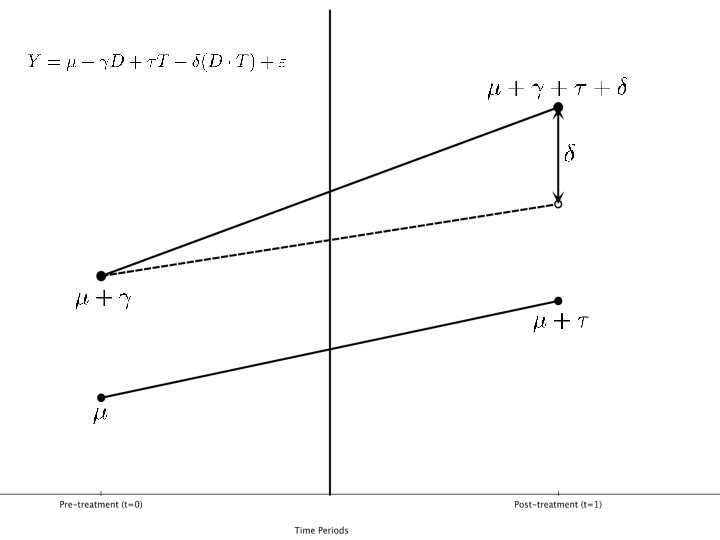
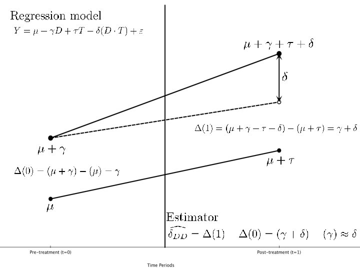
Triple DDD: Mandated Maternity Benefits (Gruber 1994)
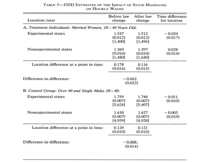
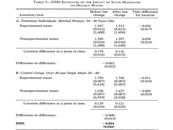

DDD Regression model

How useful is the triple DDD? • The DDD estimate is the difference between the DD of interest and the placebo DD (that is supposed to be zero) – If the placebo DD is non zero, it might be difficult to convince the reviewers that the DDD removes all the bias – If the placebo DD is zero, then DD and DDD give the same results but DD is preferable because standard errors are smaller for DD than DDD

DD: Further Threats to Validity • Functional form dependence: Magnitude or even sign of the DD effect may be sensitive to the functional form, when average outcomes for controls and treated are different at baseline – Training program for the young • Employment for the young increases from 20% to 30% • Employment for the old increases from 5% to 10% • Positive DD effect: (30 -20) – (10 -5) = 5% increase • But if you consider log changes in unemployment, the DD is [log(30) – log(20)] – [log(10)-log(5)]=log(1. 5)-log(2)<0 – DD estimates may be more reliable if treated and controls are more similar at baseline

Falsification test: placebo outcomes • Falsification test using placebo outcome that is not supposed to be affected by the treatment – If DD from placebo outcome is non-zero, then DD estimate for original outcome may be biased • Cheng and Hoekstra (2013, JHR) examine the effect of castle doctrine gun laws on homicides – They investigate the effect of the laws on non-gun related offenses, like grant theft auto, and find no evidence of an effect (“second order outcomes”) • Several studies support Becker and Murphy’s (1988) theory of rational addiction for tobacco and alcohol consumption – Auld and Grootendorst (2004, JHE) replicate the exact same models with data for milk, eggs, oranges and apples and find these plausibly non-addictive goods are addictive (casting doubt on the research design of the other studies) • Several studies have found significant networks effects on outcomes such as obesity, smoking, alcohol use, and happiness – Cohen-Cole and Fletcher (2008, BMJ) use similar models and data and find similar network “effects” for things that aren’t contagious like acne, height and headaches

Falsification test: further threats to validity • Compositional differences – One of the risks of a repeated cross-section is that the composition of the sample may have changed between periods – Example: • Hong (2011) uses repeated cross-sectional data from Consumer Expenditure Survey (CEX) containing musical expenditures and internet use for random samples of US households • Study exploits the emergence of Napster (the first sharing software widely used by Internet users) in June 1999 as a natural experiment • Study compares internet users and internet non-users, before and after emergence of Napster

Compositional differences?

Compositional differences? Diffusion of the internet changes samples (e. g. , younger music fans are early adopters)

DD: Further Threats to Validity • Long-term effects vs. reliability: – Parallel trends assumption for DD is more likely to hold over a shorter time-window – In the long-run, many other things may happen that could confound the effect of the treatment – Should be cautious to extrapolate short-term effects to long-term effects

Causal question of the day • “US abandons Effort to Place Graphic Labeling on Cigarettes” (Associated Press, March 20 2013) – US government won’t pursue a legal battle to mandate large, gruesome images on cigarette labeling in an effort to dissuade potential smokers and get current smokers to quit. – What is the causal effect of this type of “demand-side” intervention? – What data would we need to test any hypothesis relating the use of advertising on smoking? – How would we measure smoking? – What is the treatment variable? – What is the counterfactual? – What specific treatment parameter would you be trying to estimate? – How would you go about this using diff-in-diff?
, forthcoming Journal of Human Resources • English common law principle")
Cheng and Hoekstra (2013), forthcoming Journal of Human Resources • English common law principle required “duty to retreat” before using lethal force against an assailant except when the assailant is an intruder in the home – The home is one’s “castle” – hence, “castle doctrine” – When intruders threated the victim in the home, the duty to retreat was waived and lethal force in selfdefense was allowed – Very old principle predating the United States (originating in England)

“Castle doctrine law” • In 2005, Florida passed a law that expanded selfdefense protections beyond the house – 2000 to 2010, 21 states explicitly put “castle doctrine” into statute, and (more importantly) extended it to places outside the home – In other words, 21 states removed the duty to retreat in specified circumstances • Other changes: – Presumption of reasonable fear is added – Civil liability for those acting under the law is removed
, in determining")
Texas example • Duty to retreat – “For purposes of subsection (a), in determining whether an actor described by subsection (e) reasonably believed that the use of force was necessary, a finder of fact may not consider whether the actor failed to retreat. ” – Also: Language stating a person is justified using deadly force against another “if a reasonable person in the actor’s situation would not have retreated” is removed from the statute • Presumption of reasonableness – “Except as provided in subsection (b), a person is justified in using force against another when and to the degree the actor [he] reasonably believes the force is immediately necessary to protect the actor [himself] against the other’s use or attempted use of unlawful force. The actor’s belief that the force was immediately necessary as described by this subsection is presumed to be reasonable if the actor[…]” • Civil Liability – “A defendant who uses force or deadly force that is justified under Chapter 9 Penal code is immune from civil liability for personal injury or death that results from the defendant’s use of force or deadly force, as applicable. ”
 “Crime and Punishment: An Economic Approach”, Journal")
Economics of Castle Doctrine • Becker (1968) “Crime and Punishment: An Economic Approach”, Journal of Political Economy – Crime is considered to be a type of illicit labor supply with costs (foregone legal wages, risk of arrest and conviction, penalties if convicted) and benefits (plunder) – Castle doctrine laws reduce the expected costs associated with using lethal force • Therefore, we expect more lethal force due to its decrease in price
 – Increases in “true")
Economics of Castle Doctrine • More lethal force (cont. ) – Increases in “true positive” lethal force: use of lethal force against criminals committing serious crimes – Increases in “false positive” lethal force: arguments escalate to lethal force that could have been averted with “duty to retreat”; cases of mistaken identity caused by lower expected penalties for being wrong, etc. • Deterrence – Criminals, if rational, face higher expected costs and lower expected benefits (due to lower probability of success) from committing violent crimes – Therefore, economic theory suggests that depending on the elasticity of demand (e. g. , non-zero), castle doctrine will deter lethal force and thus quantity reductions – Caveat: though deterrence is a theoretical possibility, note that the goal of the laws was to protect/enhance victim rights, not deter crime
")
Castle Doctrine Laws in US, 2000 – 2010 (Table 1)

Economics concluded • Summary: – 21 states passed laws removing “duty to retreat” in places outside the home – 17 states removed “duty to retreat” in any place one had a legal right to be – 13 states include a presumption of reasonable fear – 18 states remove civil liability when force was justified under law
 – Estimates the Average Treatment")
Cheng and Hoekstra’s strategy • Research design: differences-in-differences (DD) – Estimates the Average Treatment on the Treatment Group • Identification Strategy: Compare the changes in outcomes after castle doctrine law adoption to changes in the outcomes in other states in the same region of the country • Estimation: Panel fixed effects estimation of DD parameter – Note: most of their specifications will include region dummies interacted with year dummies or “region-by-year fixed effects” which means the estimated coefficient must originate from variation within a given region (but across states within that region) in a year

Strategy • Inference: – Eleven years of data times 50 states equals 550 state units – Are disturbances random draws from individually identical distribution? It’s likely that within a state, unobserved determinants of Y are correlated over time – Bertand, Duflo and Mullainathan (2004) recommend adjusting for serial correlation in unobserved disturbances within states at the level of the treatment when estimating models in a DD research design – Cheng and Hoekstra (2013) follow common DD practice and cluster the standard errors at the state level – Additional permutation tests: “how likely is it that we estimate effects of this magnitude when using randomly chosen pre-treatment time periods and randomly assigning placebo treatments? ” • I’ve not seen this done before, so it’s interesting to me personally. It’s similar, though, to what we will see on Thursday when reviewing Abadie, et al. ’s synthetic control inference
 • Identifying assumption: absent passing castle doctrine laws, outcomes in these")
Strategy (cont. ) • Identifying assumption: absent passing castle doctrine laws, outcomes in these 21 states would have changed similar to other states in their same region – Recall the “region-by-year fixed effects” in the X term – By including “region-by-year fixed effects”, they are arguing that “parallel trends” must hold within region over time – Need not hold across regions since the across region variation is not being used in this analysis due to the saturation of the model with “region-by-year fixed effects”

Testing the identification strategy • Assess how including time-varying controls affected estimates • Examine the effect of the laws on “placebo” outcomes as a falsification (e. g. , automobile thefts and larceny) • Include state-specific linear time trends – Alabama, et al. dummy interacted with TREND which equals 1 in 2000, 2 in 2001, … , 11 in 2010 – Forces the identification to come from variation in outcomes around the statespecific linear trend • Stronger requirements, in other words • Outcomes must be large enough and different enough from a state-specific linear trend otherwise it is collinear with the state-trend • Very commonly done – personally, I find it annoying only because it’s one of many areas where DD has a tendency to become a “black box” and group trends aren’t really examined carefully enough • Include “leads” to test for divergence in the year prior to adoption • Test for historical tendency for outcomes in adopting states to diverge from control states
 – State-level crime rates, or “offenses")
Data • FBI Uniform Crime Reports (2000 -2010) – State-level crime rates, or “offenses per 100, 000 population” – Falsification outcomes: motor vehicle theft and larceny • Deterrence outcomes: – burglary: the unlawful entry of a structure to commit a felony or a theft – Robbery: the talking or attempting to take anything of value from the care, custody or control of a person or persons by force or threat of force or violence and/or putting the victim in fear – Aggravated assault: unlawful attack by one person upon another for the purpose of inflicting severe or aggravated bodily injury • Homicide categories – 1. Total homicides – murder plus non-negligent manslaughter (~14, 000 per year) – 2. Justifiable homicides by private citizens (~250/year)
 – Full-time police employment per 100,")
Data • Controls (X matrix in earlier equation) – Full-time police employment per 100, 000 state residents from the LEKOA data (FBI data) – Persons incarcerated in state prison per 100, 000 residents – Shares of white/black men in 15 -24 and 25 -44 age groups – State per capita spending on public assistance – State per capita spending on public welfare

Summary Statistics
 present falsification first to show")
Step one: Falsification test • Cheng and Hoekstra (2013) present falsification first to show the reader that they find no association within region over time in the passage of these laws and either larceny rate or motor vehicle theft rate – – • Results will be presented separately under five different specifications – • They make a big deal about the weighted vs. unweighted analysis, but I’m going to be largely ignoring this stuff as it doesn’t appear to matter What should you expect to find on key variables of interest? – – • The idea here is to immediately address concerns that what they show you later is due to generic crime trends in those states that pass the laws It’s a useful way to assuage doubt people may have, as remember, policy-makers are not just randomly flipping coins when passing laws, but presumably do so because of things they observe on the ground No statistically significant association between the CDL passage (the DD interaction) and the placebos; small magnitudes preferably too No association on the one-year lead either How do you interpret coefficients? – – His model is “log outcomes” regressed onto a dummy variable (level), so these are semi-elasticities and approximate percentage changes – but you should transform them by taking the exponential of each coefficient and then differencing it from one to find the actual percentage change Ex: CDL = -0. 0137 (column 12, Table 3, “Log (larceny rate)” outcome. Exp(-0. 0137) = 0. 986, and so 1 -0. 986 = 1. 4. Thus, CDL reduced larceny rates by 1. 4 percent, which is not statistically significant.

Results – Falsification Test

Step two: Testing Deterrence Hypothesis • Having found no effect on their placebos, Cheng and Hoekstra (2013) examine the effect of CDL on three deterrence outcomes: burglary, robbery and aggravated assault – They will, again, have five specifications per outcome in the “weighted” regression, and then another five for the “unweighted” regression • What does deterrence look like? – Negative signs on the CDL variable is consistent with deterrence – these laws are “deterred”, in other words – Bounds on the magnitudes from the standard errors are used to provide some confidence about the estimates as well

Deterrence -Lower bounds from specification 3 are -2. 1%, -1. 9%, and -2. 5% -If policy experiment were repeated many times, we’d expect 90% of the time to find deterrence effects of less than 0. 7%, 0. 4%, and 0. 5%, respectively

Conclusion about “deterrence hypothesis” • “In short, these estimates provide strong evidence against the possibility that castle doctrine laws cause economically meaningful deterrence effects” (p. 17) – Translation: They can’t find evidence of large deterrence effects • “Thus, while castle doctrine law may well have benefits to those legally justified in protecting themselves in self-defense, there is no evidence that the law provides positive spillovers by deterring crime more generally” (p. 17) – They note in footnote 24 that they cannot measure the benefits to victims whose crimes were deterred, or the benefits from lower legal costs; their focus is limited to whether it deterred the crimes, not whether the net benefits from the laws were positive – Obviously, if there is no deterrence, though, then the net benefits are lower from CDL than they would be if they did deter

Step 3: Homicides • The key finding in this study is the very large effect that CDL had on homicides and non-negligent manslaughter • As the effects are quite large, their strategy is first to present pictures • The pictures are a bit tricky, though, since they’re going to also present pictures for the control and treatment group units • This is going to be useful for eye-balling the parallel trends pre-treatment. – Remember, though – he needs parallel trends within-region – these figures don’t show that – But you should start with pictures; don’t fetishize regression

Log Homicide Rates – 2005 Adopter - Florida 105
 106")
Log Homicide Rates – 2006 Adopters (13 States) 106
 107")
Log Homicide Rates – 2007 Adopters (4 States) 107
 108")
Log Homicide Rates – 2008 Adopters (2 States) 108
 109")
Log Homicide Rates – 2009 Adopter (Montana) 109

Residual Log Homicide Rates 110

Estimation Results • Before going into the estimation results, here’s what you are looking for – This second hypothesis wherein reductions in the expected penalties and costs associated with self-defense due to CDL causes lethal violence to increase (non-deterrence escalation of violence) should exhibit a positive association on the DD variable – It should be different from zero statistically and economically meaningful • He will estimate the main DD model using panel fixed effects estimation and “negative binomial count models” – Because of the smaller number of annual homicides each year in a state, he moves away from homicide rates in some specifications and looks at “count” outcomes – He uses a class of estimators more appropriate for “counts” called “count models”, like the negative binomial estimated with maximum likelihood – Results are robust to least squares and count models

Homicide - OLS

Homicide – Negative Binomial & Murder

Homicide – Identification Test Question: Did homicide rates of adopting states show a general historical tendency to increase over time relative to other non-adopting states from the same region? Method: Move the 11 -year panel back one year at a time (covering 1960 – 2009), and estimate 40 placebo “effects” of passing castle doctrine 1 to 40 years later Findings: Method Average Estimate Weighted OLS -0. 003 Unweighted OLS 0. 001 Negative Binomial 0. 001 Estimates Larger than Actual Estimate 0/40 1/40 0/40
 Unweighted")
Homicide – Statistical Inference Tests in spirit of Bertrand, Duflo, and Mullainathan (2004) Unweighted OLS: Reject 6. 3% of the time at the 5% level => standard errors are approximately correct Weighted OLS: Reject 11. 9% of simulated estimates at the 5% level => standard errors are likely understated Negative Binomial: Reject 9. 7% of the time at the 5% level => standard errors are somewhat understated

Homicide – Statistical Inference OLS-Weighted Estimate = 0. 0946 5. 0% of placebo estimates lie to the right of the estimate;

Homicide – Statistical Inference OLS-Unweighted Estimate = 0. 0811 5. 3% of placebo estimates lie to the right of the estimate

Homicide – Statistical Inference Negative Binomial Estimate = 0. 0734 4. 6% of placebo estimates lie to the right of the estimate

Interpretation Summary: Castle Doctrine/Stand Your Ground laws lead to ~8% increase in the homicide rate Þ 600 additional homicides per year Lingering Question: Could these homicides have been misreported as murders or manslaughters, even though they actually were legally justified? Misreporting is a concern: Kleck (1988) estimates that one-fifth of legally justified homicides are correctly reported Side note: This net increase in homicides could not be driven by one-for-one substitution of would-be-homicide victims killing their assailants

Interpretation Approaches: I. Look for evidence of increases in homicides that are unambiguously unjustified (e. g. , felony murders, gang-related homicides, share of robberies with a gun, etc. ) Findings: nothing much helpful

Interpretation Approaches: II. Combine estimates of relative increase in justifiable homicides with estimates of misreporting to assess whether all the additional homicides could have been legally justified Largest estimate of relative increase in justifiable homicide: 70% Baseline number of justifiable homicides in castle doctrine states: 103 Estimate of percentage of correctly reported legally justified homicides: 20% Assumptions: i) Police are not less likely to report an otherwise identical homicide as legally justified after the passage of castle doctrine/stand-your-ground ii) The relative increase in legally justified homicides is no lower for reporting agencies than for non-reporting agencies Conclusion: At most 300 of the additional 600 homicides could have been legally justified => Some escalation of violence that is unambiguously “bad”

Conclusions • No evidence that Castle Doctrine/Stand-Your Ground Laws deter violent crimes such as burglary, robbery, and aggravated assault • These laws do lead to an 8% net increase in homicide rates, translating to around 600 additional homicides per year across the 21 adopting states Unlikely that all of the additional homicides were legally justified • Economics of crime and behavior: Incentives and expected costs appear to matter in some contexts, but not in others
")
Synthetic control Natural experiment methodologies (cont. )

Comparative Case Studies • Qualitative comparative case studies: – Goal is to reason inductively the causal effects of events or characteristics of a single unit on some outcome, but oftentimes done through logic and historical analysis • May not answer the causal inference well or at all since there is often not a counterfactual or an ad hoc counterfactual – Example: Alexis de Toqueville’s Democracy in America • De Touqueville comes to the US in the 19 th century to study our prisons • Writes classic political economy book on US institutions • Quantitative comparative case studies – Usually natural experiment methodologies applied to a single aggregate unit (e. g. , city, school, firm, state, country) – Goal is to estimate causal effect of some intervention on some outcome by comparing the evolution of the aggregate outcome in the treatment unit to the evolution of some aggregate control group

Motivating example: Mariel Boatlift How do inflows of immigrants affect the wages and employment of natives in local labor markets? Card (1990) uses the Mariel Boatlift of 1980 as a natural experiment as it caused a 7% surge in the Miami labor force due to Cuban immigration Card uses individual-level data on unemployment and wages from the Current Population Survey (CPS) for Miami and four comparison cities (Atlanta, Los Angeles, Houston and Tampa-St. Petersburg) and estimates diff-indiff History of thought: classic study because in addition to the findings, it is one of the first applications of the diff-in-diff research design and is cited in his John Bates Clark award

Motivating example: The Mariel Boatlift Differences-in-differences estimates of the effect of immigration on unemployment from Card (1990, Tables 4 columns 2 and 3) standard errors in parentheses Interpreting DD table: 1. 2. First difference (2 -1): difference across Second difference (3 a-3 b; 3 d-3 e): difference down the first difference you computed in part 1 (You can also difference down then across – same answer either way) Estimated average treatment effect on the treatment group is -1. 1 for Whites and -1. 0 for Blacks. Conclusion: Mariel Boatlift-induced immigration reduced unemployment by 1 percentage point Group 1979 (1) 1981 (2) 1981 -1979 (3) (a) Miami 5. 1 (1. 1) 3. 9 (0. 9) -1. 2 (1. 4) (b) Comparison cities 4. 4 (0. 3) 4. 3 (0. 3) -0. 1 (0. 4) (c) Difference Miami-comparison 0. 7 (1. 1) -0. 4 (0. 95) -1. 1 (1. 5) (d) Miami 8. 3 (1. 7) 9. 6 (1. 8) 1. 3 (2. 5) (e) Comparison cities 10. 3 (0. 8) 12. 6 (0. 9) 2. 3 (1. 2) (f) Difference Miami-comparison -2. 0 (1. 9) -3. 0 (2. 0) -1. 0 (2. 8) Whites Blacks
 identifies the average treatment effect on the")
Identifying assumptions in DD • Differences-in-differences (DD) identifies the average treatment effect on the treatment group (ATT) parameter: – Definition of ATT: E[Y 1|D=1, T=1] – E[Y 0|D=1, T=1] – Second term is “counterfactual” – it never occurred and is therefore unobserved • DD research designs require strong (untestable) assumptions about counterfactual time paths treatment group outcomes (Y) – Parallel trends assumption: Rate of change in Y for control group from pre- to post-treatment period equals rate of change in Y for treatment group from pre- to post-treatment period had treatment not been assigned (counterfactual) – E[Y 0|D=1, T=1]–E[Y 0|D=1, T=0]=E[Y 0|D=0, T=1]–E[Y 0|D=0, T=0]
")
Identification in DD (Graphical)
 select Los Angeles, Tamp, Houston and Atlanta")
Selection of controls How did Card (1990) select Los Angeles, Tamp, Houston and Atlanta as comparison cities? “These four cities were selected because they had relatively large populations of blacks and Hispanics and because they exhibited a pattern of economic growth similar to that in Miami over the late 1970 s and early 1980 s. ” Implicit assumption in choosing four cities: Change in average unemployment for Miami from 1979 to 1981 had Mariel Boatlift never occurred (counterfactual trend) equals Change in average unemployment for ATL, HOU, Tampa and LA from 1979 to 1981 (observed trend) Are demographics predictive of the outcome of interest pre-treatment? Does Card’s synthetic Miami reproduce the time-path of Miami in earlier periods?

Advantages and disadvantages • What are the advantages of comparative case studies? – Policy interventions often take place at an aggregate level – Aggregate/macro data are often available • What are the disadvantages? – Selection of the control group is often ambiguous (e. g. , Card 1990) – Standard errors do not reflect uncertainty about the ability of the control group to reproduce the counterfactual of interest • Split the difference with synthetic control method – Same advantages, fewer of the disadvantages

The Synthetic Control Method • Key papers for further reading – Abadie and Gardeazabal (2003) “The Economic Costs of Conflict: A Case Study of the Basque Country”, American Economic Review, 93(1), March 113 -132 – Abadie, Diamond and Hainmueller (2010) “Synthetic Control Methods for Comparative Case Studies: Estimating the Effect of California’s Tobacco Control Program”, Journal of the American Statistical Association, 105(490), June, 493 -505. – Abadie, Diamond and Hainmueller (2011) “Synth: An R Package for Synthetic Control Methods in Comparative Case Studies”, Journal of Statistical Software, 42(13), June, 2 -17. – Abadie, Diamond and Hainmueller (2012) “Comparative Politics and the Synthetic Control Method”, Unpublished manuscript

Basic ideas • When to use synthetic control: causal inference questions, aggregate data, one treatment unit – You are interested in the causal effect of some intervention on some outcome of interest • Ex: School choice on academic performance – Units are aggregate (e. g. , school, firm, country, state, region) as opposed to samples of the population • Census longform is a 10% sample of the US population (sampling uncertainty) • Administrative records for students at A&M is aggregate (no sampling uncertainty) – Treatment assignment is aggregate and affects one unit • Ex: Massachusett’s healthcare reform only in MA, and affected all of Massachusett
 • Key concept: composites can be better mimics than individual")
Basic Ideas (cont. ) • Key concept: composites can be better mimics than individual comparisons – We can often reproduce the characteristics of a unit(s) using combinations of control units than trying to find the perfect one unit for comparison • Example: What’s the effect of RG 3 winning the Heisman on Baylor student academic achievement and enrollment? • Problem: Who is like Baylor? ? • Solution: “Frankenstein Baylor” – combine 4 -5 other schools vs. trying to find the “perfect other school” – Synthetic control method optimally selects weights to create “Frankenstein” versions of the treatment group • Weights are optimal in that they are selected by an algorithm using pre-treatment data and a reservoir of control group units such that the “Frankenstein” looks and acts like the treatment group prior to the intervention – Weights are selected based on pre-treatment data only, but causal inference is based on comparing the fit of the model post-to-pre treatment • Baylor outcomes: pre-RG 3 vs. “Frankenstein Baylor” pre-RG 3. Hopefully they look very similar • Baylor outcomes: post-RG 3 vs. “Frankenstein Baylor” post-RG 3. Their difference is the estimated causal effect of RG 3 on that event – Assumes no spill-overs from treatment onto controls, including no general equilibrium effects • More appropriate, probably, for short-run shocks – Inference method is demanding, and so causal effects must be large enough

Synthetic Control: Advantages • Advantages – Doesn’t extrapolate beyond support of data • Estimated counterfactual is a convex combination of other units’ outcome, which precludes extrapolation beyond the support of the data • OLS extrapolates beyond the support of the data – Transparency • Synthetic control produces a vector of weights – you know precisely who forms your counterfactual and by how much • OLS is a black box by comparison even though it also creates implicit weights – Builds on other comparative case study practices • Allows for a mixture of qualitative and quantitative methods – e. g. , if Arizona contributes 50% to your synthetic Rhode Island unit, you know to scrutinize Arizona to try and better understand why pretreatment the two units performed so well together – Reduced opportunity for subjective researcher bias • Synthetic control formalizes the selection of comparison units and therefore removes the temptation of researchers to endogenously choose comparison cities based on either ad hoc reasoning and/or researcher biases – Inference • Represents not only a formal way of systematizing comparative case studies, but it also provides a permutation-based method of inference for quantifying uncertainty

Synthetic control: disadvantages • Audience ignorance can be a problem since this is new and competes with DD – While this is changing, quite common to be met with skepticism by practioners who prefer diff -in-diff for no other reason that they are familiar with it – Means synthetic control is still viewed as a “robustness” check, as opposed to the principal design used in program evaluation – Level of problem: not a big deal, and won’t matter if you do this in addition to everything else (which you should be doing anyway) • Volatility in pre-treatment series can cause you to never find a suitable synthetic control – Level of problem: bigger deal in a sense, but should you be using DD if you learn from synthetic control that there doesn’t exist any composite that can reproduce your treatment group? Wouldn’t you rather know, in other words, than just run regressions? • Lots of model fitting – Although you are model fitting on the pre-treatment series, and thus technically this is done prior to the actual estimation itself, -synth- and other packages does this in one swoop thus defeating in some sense one of the motivating purposes of the procedure which is to reduce researcher bias – Level of problem: in my opinion, probably the biggest “black box” part of synthetic control

Synthetic control method: Formalization • • Suppose J+1 units in periods 1, 2, …, T Unit “one” is the treatment group unit (“treated”) exposed to the intervention of interest during periods T 0+1, …, T – – • • Remaining J units are called the “donor pool” as they are the untreated reservoir of potential controls Goal is to find a combination of untreated units from the donor pool (J) that resemble the treated unit (j=1) prior to the intervention in terms of k relevant covariates (predictors of the outcome of interest) – • Ex: 49 control states and 1 treatment state; J=49 plus the 1 treatment state is 50 states T 0 in this notation is the number of pre-treatment time periods (e. g. , 10 periods pre-treatment, so T 0=10). User can choose to include as many as M linearly independent combinations of pre-intervention outcomes so long as M is less than or equal to T 0 to control for unobserved common factors Today’s motivating example: 1988 California’s tobacco control program – – – Treatment unit is California Treatment is Proposition 99 Outcome of interest is tobacco consumption in California after 1988 Donor pool is all states that did not receive similar legislation during this period Covariates are the predictors of state-level tobacco consumption measured before 1988

Synthetic control method: Formalization • Consider a set of weights w 2, …, w. J+1, where the following criteria hold: – Each weight is non-negative (0 or positive) – Weights must sum to 1 • Estimation of weights: constrained minimization – Let Xjm be the value of the mth covariates for unit j – Choose w*2, … , w*J+1 that minimizes the following (subject to above constraints): – V is defined as some (k x k) symmetric and positive semidefinite matrix • V is introduced to allow different weights to the variables in X 0 and X 1 depending on their predictive power on the outcome Y • An optimal choice of V assigns weights that minimize the mean square error of the synthetic control estimator, that is the expectation of ( Y 1 -Y 0 W*)’(Y 1 -Y 0 W*)
 propose a data-driven procedure to choose")
Optimal V matrix • Abadie, et al. (2010) propose a data-driven procedure to choose V, and this is implemented by default in – synth– • V* is chosen among all positive definite and diagonal matrices such that the mean squared prediction error (MSPE) of the outcome variable is minimized over some set of pre-treatment periods – Let Z 1 be a vector with the values of the outcome variable for the treatment unit for some set of pre-intervention periods – Let Z 0 be an analogous matrix for the control units – The user will choose the number of pre-intervention periods over which the MSPE is minimized

Optimal V matrix • Choose V* that minimizes the following expression where V is the set of all positive definite and diagonal matrices and the weights for the synthetic control are given by W* from the earlier slide

Synthetic Control Method: Formalization • Let Yjt be the value of the outcome for unit j at time t • Weights are applied outcomes and causal effects are differences between actual outcome and synthetic control outcome, or “prediction gap” • The causal effect you are estimating with synthetic control is, like DD, the average treatment effect on the treatment group (not the average treatment effect, in other words)

What about selection on unobservables? • Selection on unobservables: just because two units look the same doesn’t mean they are the same in ways that are relevant to the outcome of interest – Unmeasured factors affecting outcome variables, heterogeneity in the effect itself and treatment selection is problematic as always • Include lagged dependent variables as controls in the X matrix, but you will need a lot of pre-treatment data – Abadie, Diamond and Hainmueller (2010) argue that if the number of preintervention periods in the data is large, then matching on pre-intervention outcomes, Y, allows us to control for heterogeneous responses to multiple unobserved factors • What’s the intuition here? – Assume outcomes (Y) are a function of observables (X) and unobservables (u) – By matching on Y pre-treatment, we are incorporating X and u – Only units that are alike in both observed X and unobserved u as well as in the effect of those determinants on Y should produce similar trajectories of the outcome variable over extended periods of time

The Application: California’s Proposition 99 • In 1988, California first passed comprehensive tobacco control legislation: – – – Increased cigarette tax by 25 cents/pack Earmarked tax revenues to health and anti-smoking budgets Funded anti-smoking media campaigns Spurred clean-air ordinances throughout the state Produced more than $100 million per year in anti-tobacco projects • Other states that subsequently passed control programs will be excluded from their analysis by eliminating these states from the “donor pool” – AK, AZ, FL, HA, MD, MI, NJ, NY, OR, WA, DC all dropped

Cigarette Consumption: CA vs US

Cigarette consumption: CA vs. Synthetic CA

Predictor Means: Actual vs. Synthetic CA

Smoking Gap: CA vs. Synthetic CA

Inference • So what? – I still don’t know how confident to be about these post-estimation estimates of causal effects unless I have some way of quantifying the uncertainty • What kind of uncertainty, though, ultimately are worried about? – Counterfactual uncertainty. The fundamental problem of causal inference is that we do not have counterfactuals on individual units, and therefore cannot directly measure causal effects • Cannot observe California and smoking in the counterfactual state – Randomness. Secondly, related to this, for all we know, this model produces a picture just like the previous ones even if it’s applied to states that didn’t pass Proposition 99 • In other words, maybe synthetic control models fitted with pre-treatment data always dissolve like that – in which case, that picture isn’t so convincing anymore

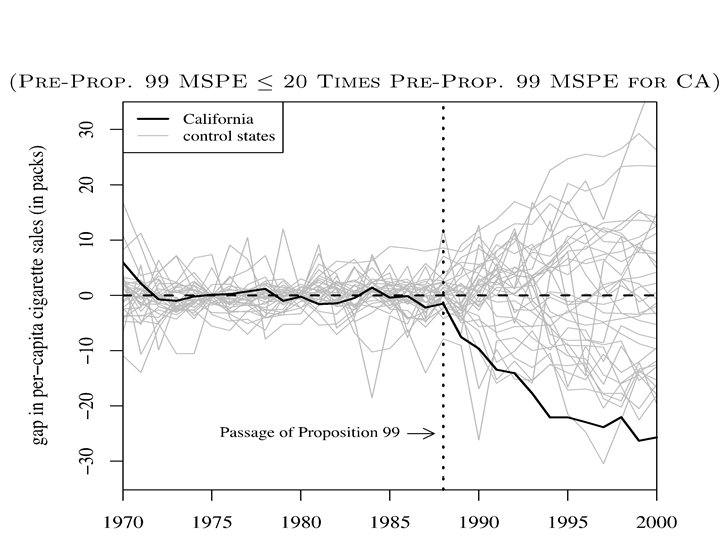
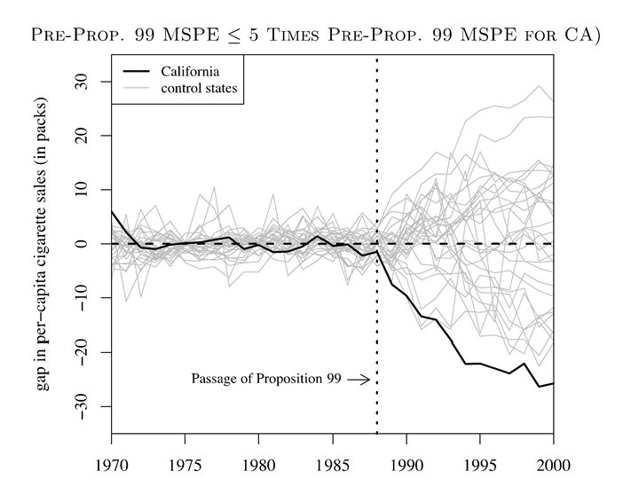
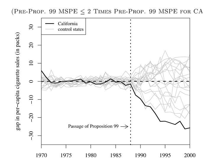
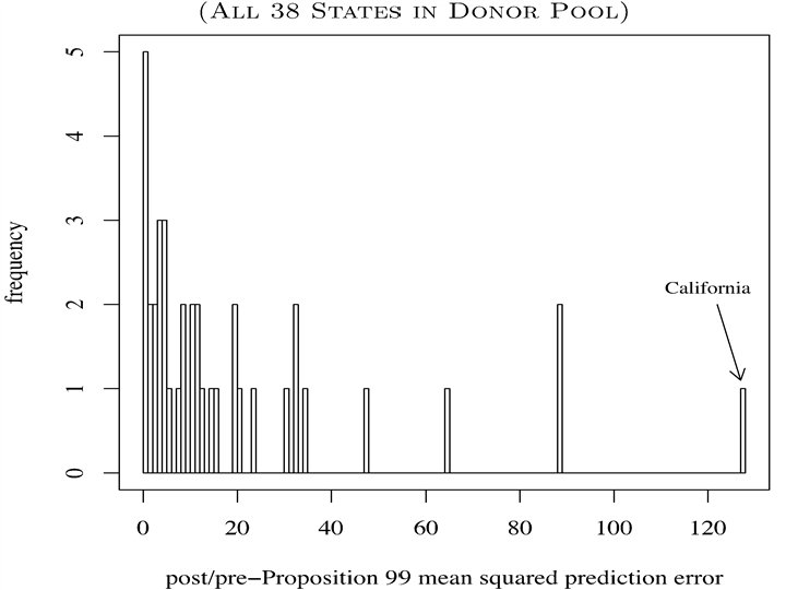
Inference • To evaluate the significance of our results using synthetic control, we will conduct a series of “placebo” experiments where we reassign the tobacco control program to states other than California – 1. Iteratively apply the synthetic method to each unit in our “donor pool” to obtain a distribution of these “placebo effects” – 2. Compare the “prediction gap” (RMSPE) for California to the entire distribution of these estimated “placebo effects” – 3. Is the effect that we estimated with synthetic control for California large relative to the “placebo effects” we estimated for a state chosen at random?

Smoking prediction gap for CA and 38 placebos
 the authors propose more applications,")
Further falsification exercises • In Abadie, et al. (2012) the authors propose more applications, but more importantly for us, more robustness exercises • We will consider primarily two of them: – Shifting the treatment data within treatment group – Removing units from the synthetic control

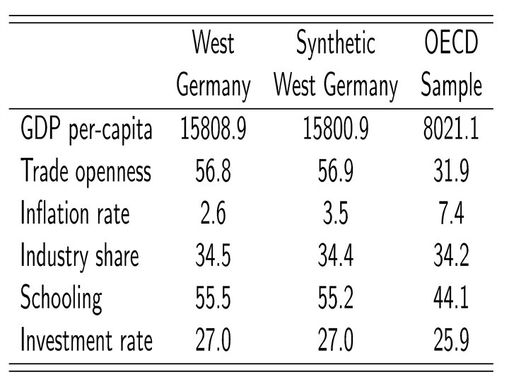
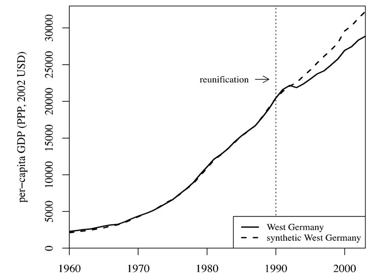
Application 2: The 1990 German Reunification • Cross-country regressions are often criticized because they put side -by-side countries of very different characteristics • “What do Thailand, the Dominican Republic, Zimbabwe, Greece, and Bolivia have in common that merits their being put in the same regression analysis? Answer: For most purposes, nothing at all. ” (Harberger, 1987). • The synthetic control method provides us with a data-driven procedure for selecting the appropriate comparison units, thereby addressing Harberger’s complaints • Application: examine the economic impact of the 1990 German reunification in West Germany – Abadie, Diamond and Hainmueller (2012), unpublished manuscript – They limit the donor pool to 16 OECD countries

West Germany vs OECD sample
 in the synthetic control")
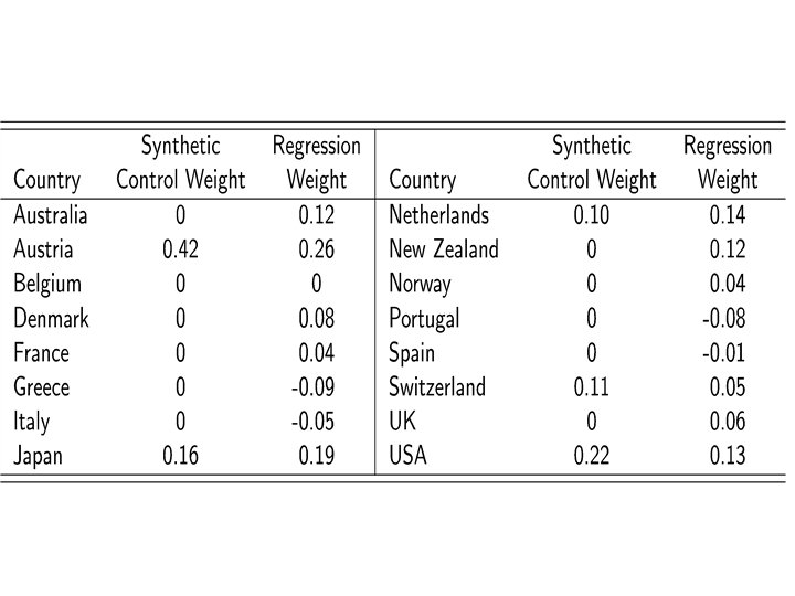
Country weights (w*) in the synthetic control

Comparison to Regression • Constructing a synthetic comparison as a linear combination of the untreated units with coefficients that sum to one may appear to many as unusual • Abadie, Diamond and Hainmueller (2012) prove, though, that regression-based approaches actually do this very same thing albeit in an implicit way • Unlike synthetic control methods, regression approaches do not restrict the coefficients of the linear combination that define the comparison units to be in between zero and one – As a result, regression-based approaches allow extrapolation beyond the support of the data

Robustness I: Placebo reunification: 1975

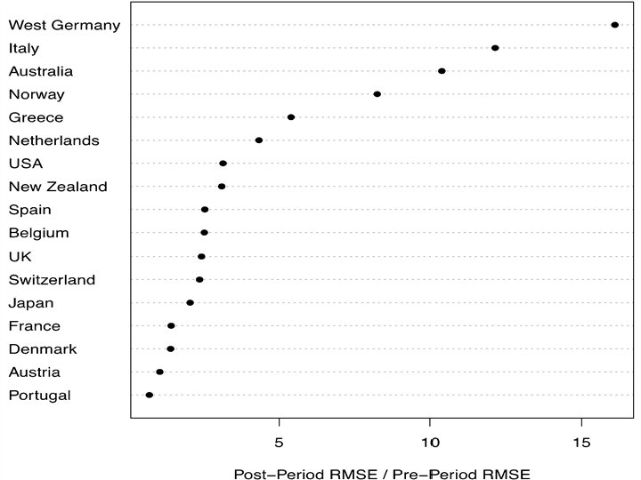
Robustness II: Leave-on-out distribution

Sparse Synthetic Controls

Sparse Synthetic Controls

Synthetic Control with 5 Countries

Synthetic Control with 4 countries

Synthetic control with 3 countries

Synthetic control with 2 countries

Synthetic control with 1 country
 is available for STATA")
STATA and R resources • Abadie, Diamond and Hainmueller (2010) is available for STATA and R in a package called “synth” – STATA: . ssc install synth, replace – R: http: //www. jstatsoft. org/v 42/i 13 • Permutation-based inference procedure may need to be manually done, though, as their help file documentation has never worked for me (I’m probably just not smart enough) – See my do file from my project on the decriminalization of indoor prostitution and its effect on rapes
")
Instrumental Variables Natural experiment methodologies (cont. )

IV Background: Slide 1 • Many empirical papers seeking to address the causal effect of one variable (X) on another (Y) will begin by regressing Y on X: –. reg workforpay numkids • • For the regression to give a reliable answer to the question of causality, the data must satisfy core assumptions These assumptions have lots of different flavors as we’ve seen so far. Here is one example of those assumptions: if X is randomly assigned to units, then the regression of Y on X gives a good estimate of what would happen on average if we manipulated a given observation to have a different value of X than it did in reality – In other words, the coefficient on X (numkids) would give us an estimate of the counterfactual because, in reality, the manipulation of X was not what happened – Ex: suppose the 10 th observation (“Julie Smith”) had X 10=0 and we wondered what would happen if that 10 th observation (“Julie”) was manipulated so that she had actually had X 10=1. Even though Julie only had X 10=0, if X was randomly assigned to units, the coefficient on the regression would give us the effect of a one unit increase in X on Y – on average – across the units in the study • So… what is the regression telling us when X was not randomly assigned?

IV Background: Slide 2 • Let the kx 1 regression coefficient vector, , be defined by solving the following equation: • Using the first order conditions, we • The coefficient on X in “reg Y X” is an estimate of:
- Slides: 175