Selecting Input Probability Distribution Simulation Machine Simulation can

Selecting Input Probability Distribution

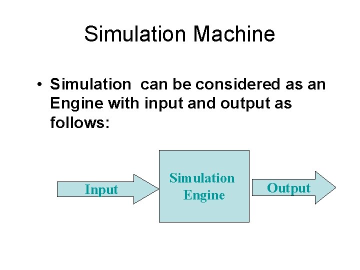
Simulation Machine • Simulation can be considered as an Engine with input and output as follows: Input Simulation Engine Output

Realizing Simulation • Input Analysis: is the analysis of the random variables involved in the model such as: – The distribution of IAT – The distribution of Service Times • Simulation Engine is the way of realizing the model, this includes: – Generating Random variables involved in the model – Performing the requiring formulas. • Output Analysis is the study of the data that are produced by the Simulation engine.

Input Analysis • collect data from the field • Analyze these data • Two ways to analyze the data: – Build Empirical distribution and then sample from this distribution. – Fit the data to a theoretical distribution ( such as Normal, Exponential, etc. ) See Chapter 6 of Text for more distributions.

How to select an Input Probability distribution 1. Hypothesize a family of distributions. 2. Estimate the parameters of the fitted distributions 3. Determine how representative the fitted distributions are 4. Repeat 1 -3 until you get a fitted distribution foe the collected data. Otherwise go with an empirical distribution.

Hypothesizing a Theoretical Distribution To Fit a Theoretical Distribution • Need a good background of theoretical distributions (Consult your Text: Section 6. 2) • Histogram may not provide much insight into the nature of the distribution. • Need Summary statistics

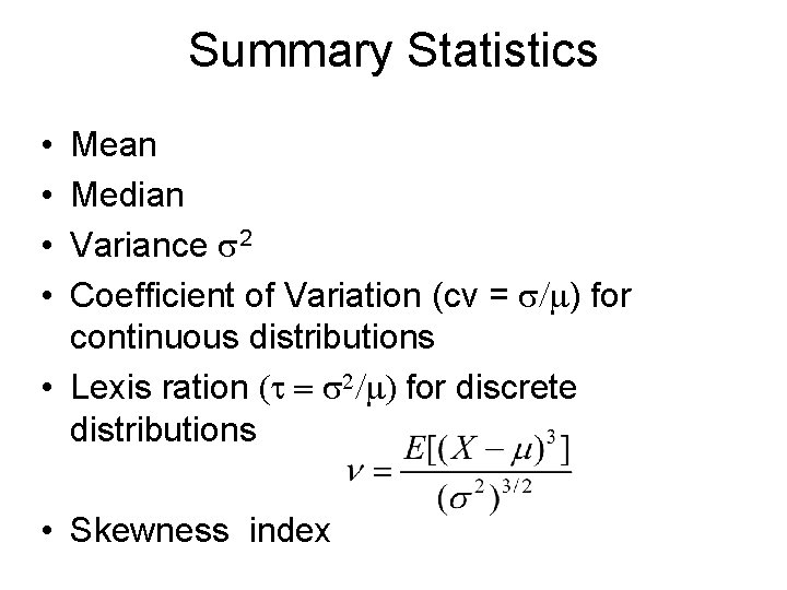
Summary Statistics • • Mean Median Variance s 2 Coefficient of Variation (cv = s/m) for continuous distributions • Lexis ration (t = s 2/m) for discrete distributions • Skewness index

Summary Stats. Cont. • If the Mean and the Median are close to each others, and low Coefficient of Variation, we would expect a Normally distributed data. • If the Median is less than the Mean, and s is very close to the Mean (cv close to 1), we expect an exponential distribution. • If the skewness (n close to 0) is very low then the data are symmetric.

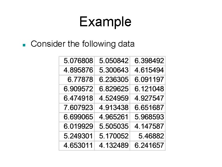
Example n Consider the following data

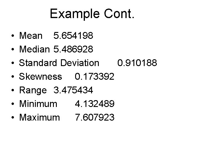
Example Cont. • • Mean 5. 654198 Median 5. 486928 Standard Deviation 0. 910188 Skewness 0. 173392 Range 3. 475434 Minimum 4. 132489 Maximum 7. 607923

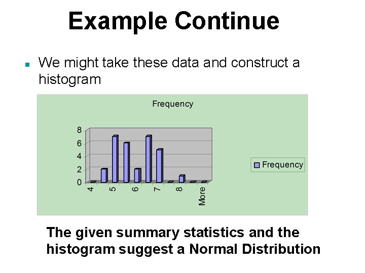
Example Continue n We might take these data and construct a histogram The given summary statistics and the histogram suggest a Normal Distribution

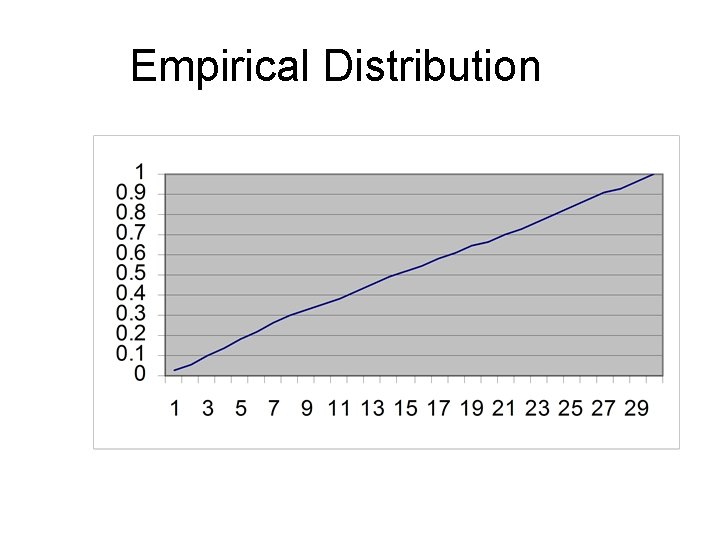
Empirical Distribution

Disadvantages of Empirical distribution • The empirical data may not adequately represent the true underlying population because of sampling error • The Generated RV’s are bounded • To overcome these two problems, we attempt to fit a theoretical distribution.

Estimation of Parameters of the fitted distributions Suppose we hypothesized a distribution, then use the Maximum Likelihood Estimator (MLE) to estimate the parameters involved with the hypothesized distribution. • Suppose that q is the only parameter involve in the distribution then construct (for example the mean 1/l in the exponential distribution) • Let L(q) = fq (X 1) fq (X 2). . . fq(Xn) • Find q that maximize L(q) to be the required parameter. • Example: the exponential distribution. Do in class

Determine how representative the fitted distributions are • Goodness of Fit (Chi Squared method)

Goodness of Fit (Chi Square method) 1. Divide the range of the fitted distribution into k (k<30) intervals [a 0, a 1), [a 1, a 2), … [ak-1, ak] Let Nj = the number of data that belong to [aj-1, aj) 2. Compute the expected proportion of the data that fall in the jth interval using the fitted distribution call them pj 3. Compute the Chi-square

Chi-square cont. • Note that npj represents the expected number of data that would fall in the jth interval if the fitted distribution is correct. • If • Where r is the number of parameters in the distribution (in Exponential dist. r = 1 which is l) • Then do not reject distribution with significance (1 -a)100%.

Example: • Consider the following data: 0. 01, 0. 07, 0. 03, 0. 23, 0. 04, 0. 10, 0. 31, 1. 17, 1. 50, 0. 93, 1. 54, 0. 19, 0. 17, 0. 36, 0. 27, 0. 46, 0. 51, 0. 11, 0. 56, 0. 72, 0. 39, 0. 04, 0. 78 Suppose we hypothesize an exponential distribution, Use Chi-square test by dividing the range into 5 subintervals.

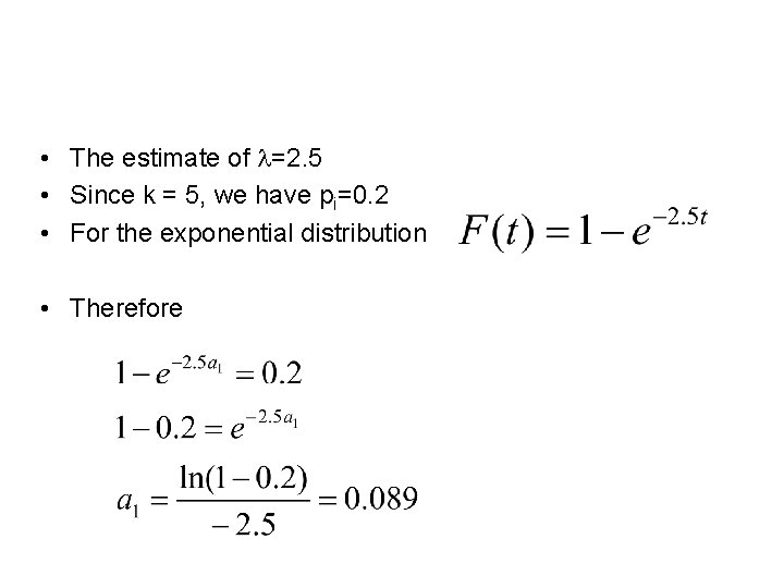
• The estimate of l=2. 5 • Since k = 5, we have pi=0. 2 • For the exponential distribution • Therefore

• Therefore chi-square = 0. 4 • From the tables of chi-square • we can accept the hypothesis With significance level 5%

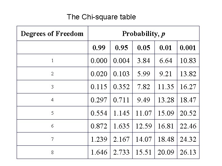
The Chi-square table Degrees of Freedom Probability, p 0. 99 0. 95 0. 01 0. 001 1 0. 000 0. 004 3. 84 6. 64 10. 83 2 0. 020 0. 103 5. 99 9. 21 13. 82 3 0. 115 0. 352 7. 82 11. 35 16. 27 4 0. 297 0. 711 9. 49 13. 28 18. 47 5 0. 554 1. 145 11. 07 15. 09 20. 52 6 0. 872 1. 635 12. 59 16. 81 22. 46 7 1. 239 2. 167 14. 07 18. 48 24. 32 8 1. 646 2. 733 15. 51 20. 09 26. 13