SEISMIC SURFACE WAVE TOMOGRAPHY ON DENSE 3 D

SEISMIC SURFACE WAVE TOMOGRAPHY ON DENSE 3 D ACTIVE DATA EGU 2020 Ilaria Barone Emanuel Kästle Claudio Strobbia Giorgio Cassiani Università degli Studi di Padova realtimeseismic

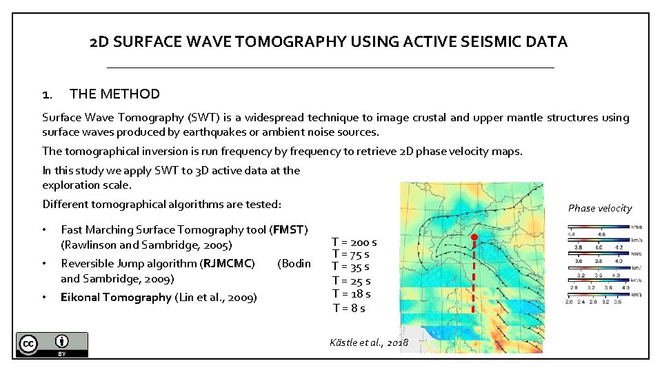
2 D SURFACE WAVE TOMOGRAPHY USING ACTIVE SEISMIC DATA 1. THE METHOD Surface Wave Tomography (SWT) is a widespread technique to image crustal and upper mantle structures using surface waves produced by earthquakes or ambient noise sources. The tomographical inversion is run frequency by frequency to retrieve 2 D phase velocity maps. In this study we apply SWT to 3 D active data at the exploration scale. Different tomographical algorithms are tested: • Fast Marching Surface Tomography tool (FMST) (Rawlinson and Sambridge, 2005) • Reversible Jump algorithm (RJMCMC) and Sambridge, 2009) • Eikonal Tomography (Lin et al. , 2009) (Bodin Phase velocity T = 200 s T = 75 s T = 35 s T = 25 s T = 18 s T=8 s Kästle et al. , 2018

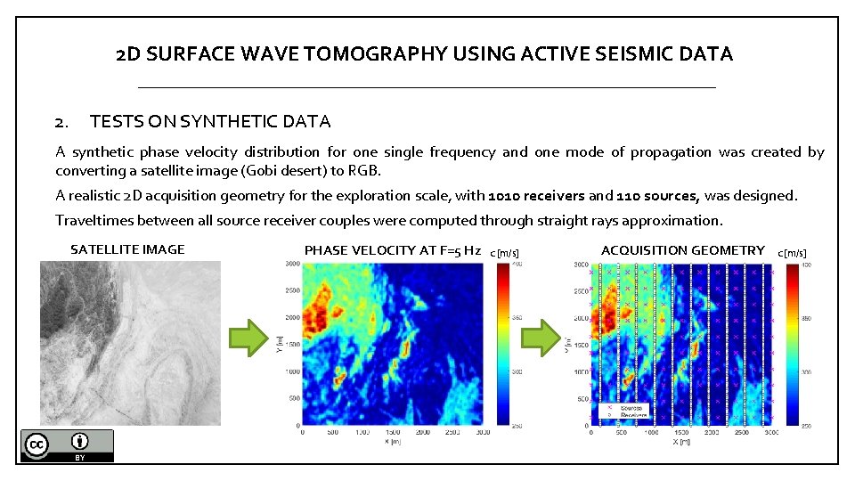
2 D SURFACE WAVE TOMOGRAPHY USING ACTIVE SEISMIC DATA 2. TESTS ON SYNTHETIC DATA A synthetic phase velocity distribution for one single frequency and one mode of propagation was created by converting a satellite image (Gobi desert) to RGB. A realistic 2 D acquisition geometry for the exploration scale, with 1010 receivers and 110 sources, was designed. Traveltimes between all source receiver couples were computed through straight rays approximation. SATELLITE IMAGE PHASE VELOCITY AT F=5 Hz c [m/s] ACQUISITION GEOMETRY c [m/s]

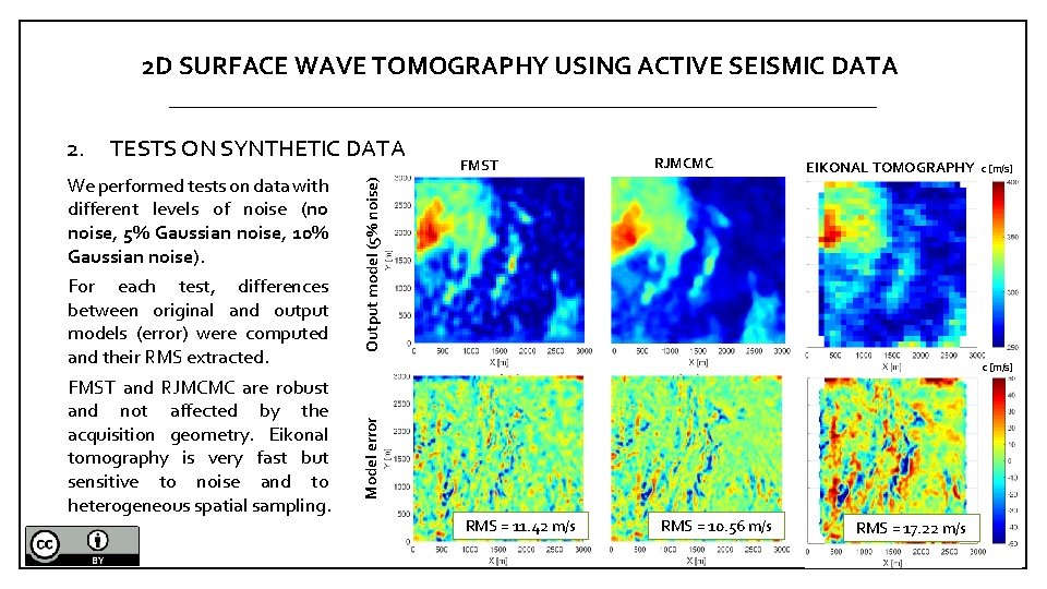
2 D SURFACE WAVE TOMOGRAPHY USING ACTIVE SEISMIC DATA We performed tests on data with different levels of noise (no noise, 5% Gaussian noise, 10% Gaussian noise). For each test, differences between original and output models (error) were computed and their RMS extracted. FMST and RJMCMC are robust and not affected by the acquisition geometry. Eikonal tomography is very fast but sensitive to noise and to heterogeneous spatial sampling. FMST RJMCMC EIKONAL TOMOGRAPHY c [m/s] Output model (5% noise) TESTS ON SYNTHETIC DATA c [m/s] Model error 2. RMS = 11. 42 m/s RMS = 10. 56 m/s RMS = 17. 22 m/s

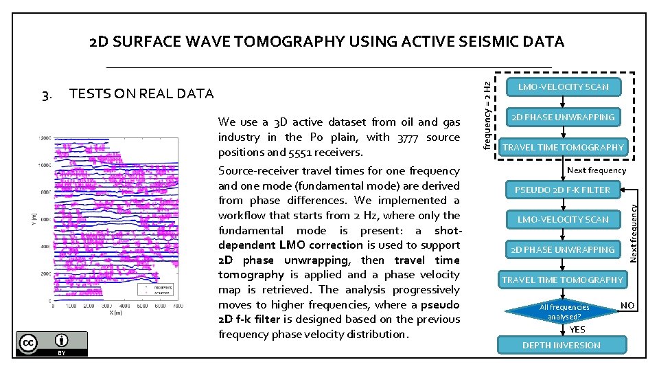
TESTS ON REAL DATA We use a 3 D active dataset from oil and gas industry in the Po plain, with 3777 source positions and 5551 receivers. Source-receiver travel times for one frequency and one mode (fundamental mode) are derived from phase differences. We implemented a workflow that starts from 2 Hz, where only the fundamental mode is present: a shotdependent LMO correction is used to support 2 D phase unwrapping, then travel time tomography is applied and a phase velocity map is retrieved. The analysis progressively moves to higher frequencies, where a pseudo 2 D f-k filter is designed based on the previous frequency phase velocity distribution. LMO-VELOCITY SCAN 2 D PHASE UNWRAPPING TRAVEL TIME TOMOGRAPHY Next frequency PSEUDO 2 D F-K FILTER Next frequency 3. frequency = 2 Hz 2 D SURFACE WAVE TOMOGRAPHY USING ACTIVE SEISMIC DATA LMO-VELOCITY SCAN 2 D PHASE UNWRAPPING TRAVEL TIME TOMOGRAPHY All frequencies analysed? YES DEPTH INVERSION NO

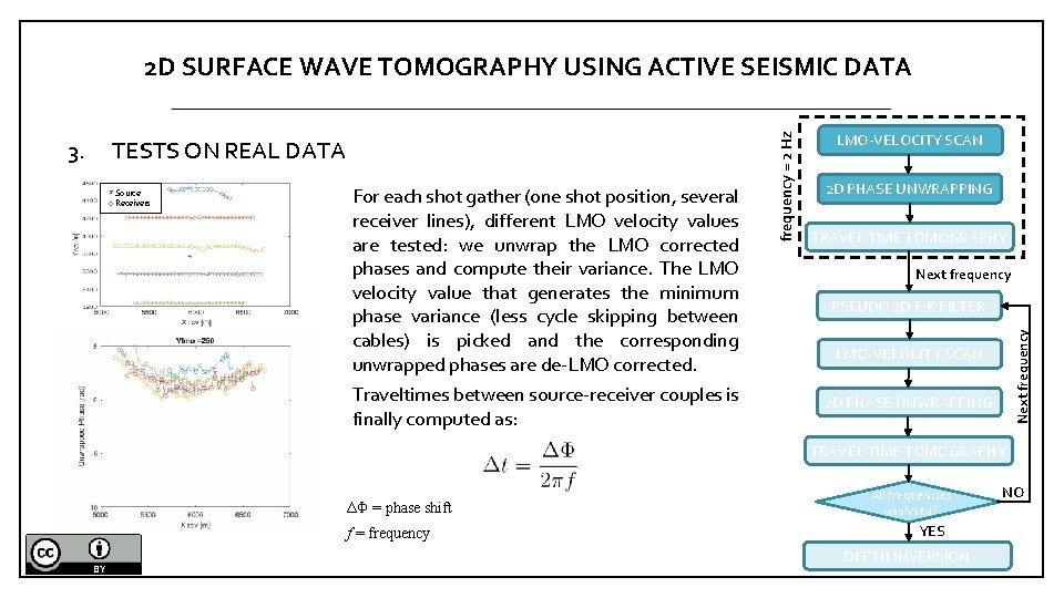
TESTS ON REAL DATA * Source o Receivers For each shot gather (one shot position, several receiver lines), different LMO velocity values are tested: we unwrap the LMO corrected phases and compute their variance. The LMO velocity value that generates the minimum phase variance (less cycle skipping between cables) is picked and the corresponding unwrapped phases are de-LMO corrected. Traveltimes between source-receiver couples is finally computed as: LMO-VELOCITY SCAN 2 D PHASE UNWRAPPING TRAVEL TIME TOMOGRAPHY Next frequency PSEUDO 2 D F-K FILTER Next frequency 3. frequency = 2 Hz 2 D SURFACE WAVE TOMOGRAPHY USING ACTIVE SEISMIC DATA LMO-VELOCITY SCAN 2 D PHASE UNWRAPPING TRAVEL TIME TOMOGRAPHY ΔΦ = phase shift f = frequency All frequencies analysed? YES DEPTH INVERSION NO

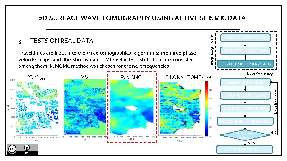
TESTS ON REAL DATA Traveltimes are input into the three tomographical algorithms: the three phase velocity maps and the shot-variant LMO velocity distribution are consistent among them. RJMCMC method was chosen for the next frequencies. 2 D VLMO FMST RJMCMC EIKONAL TOMO c [m/s] LMO-VELOCITY SCAN 2 D PHASE UNWRAPPING TRAVEL TIME TOMOGRAPHY Next frequency PSEUDO 2 D F-K FILTER Next frequency 3. frequency = 2 Hz 2 D SURFACE WAVE TOMOGRAPHY USING ACTIVE SEISMIC DATA LMO-VELOCITY SCAN 2 D PHASE UNWRAPPING TRAVEL TIME TOMOGRAPHY All frequencies analysed? YES DEPTH INVERSION NO

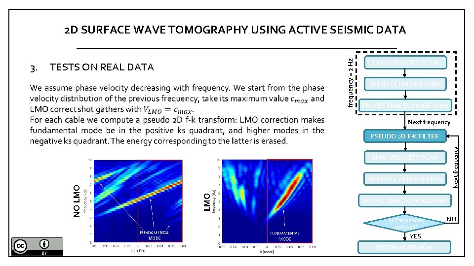
TESTS ON REAL DATA LMO-VELOCITY SCAN 2 D PHASE UNWRAPPING TRAVEL TIME TOMOGRAPHY Next frequency PSEUDO 2 D F-K FILTER LMO-VELOCITY SCAN LMO 2 D PHASE UNWRAPPING NO LMO 3. frequency = 2 Hz 2 D SURFACE WAVE TOMOGRAPHY USING ACTIVE SEISMIC DATA TRAVEL TIME TOMOGRAPHY All frequencies analysed? YES DEPTH INVERSION NO

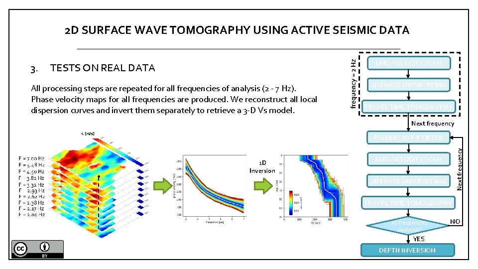
TESTS ON REAL DATA All processing steps are repeated for all frequencies of analysis (2 - 7 Hz). Phase velocity maps for all frequencies are produced. We reconstruct all local dispersion curves and invert them separately to retrieve a 3 -D Vs model. LMO-VELOCITY SCAN 2 D PHASE UNWRAPPING TRAVEL TIME TOMOGRAPHY Next frequency c [m/s] PSEUDO 2 D F-K FILTER 1 D Inversion Next frequency 3. frequency = 2 Hz 2 D SURFACE WAVE TOMOGRAPHY USING ACTIVE SEISMIC DATA LMO-VELOCITY SCAN 2 D PHASE UNWRAPPING TRAVEL TIME TOMOGRAPHY All frequencies analysed? YES DEPTH INVERSION NO

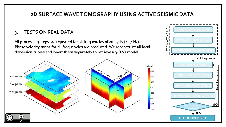
TESTS ON REAL DATA All processing steps are repeated for all frequencies of analysis (2 - 7 Hz). Phase velocity maps for all frequencies are produced. We reconstruct all local dispersion curves and invert them separately to retrieve a 3 -D Vs model. LMO-VELOCITY SCAN 2 D PHASE UNWRAPPING TRAVEL TIME TOMOGRAPHY Next frequency PSEUDO 2 D F-K FILTER Next frequency 3. frequency = 2 Hz 2 D SURFACE WAVE TOMOGRAPHY USING ACTIVE SEISMIC DATA LMO-VELOCITY SCAN 2 D PHASE UNWRAPPING TRAVEL TIME TOMOGRAPHY All frequencies analysed? YES DEPTH INVERSION NO