SEGMENTATION By Zvi solomon Seri khoury Lecturer Hagit

SEGMENTATION By Zvi solomon & Seri khoury Lecturer : Hagit Hel-Or

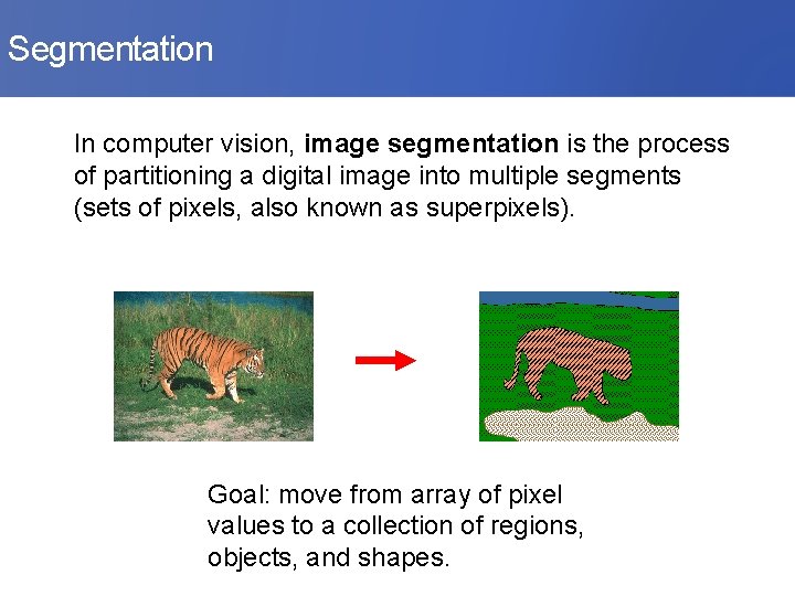
Segmentation In computer vision, image segmentation is the process of partitioning a digital image into multiple segments (sets of pixels, also known as superpixels). Goal: move from array of pixel values to a collection of regions, objects, and shapes.

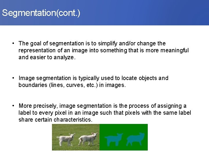
Segmentation(cont. ) • The goal of segmentation is to simplify and/or change the representation of an image into something that is more meaningful and easier to analyze. • Image segmentation is typically used to locate objects and boundaries (lines, curves, etc. ) in images. • More precisely, image segmentation is the process of assigning a label to every pixel in an image such that pixels with the same label share certain characteristics.

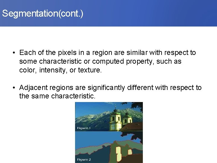
Segmentation(cont. ) • Each of the pixels in a region are similar with respect to some characteristic or computed property, such as color, intensity, or texture. • Adjacent regions are significantly different with respect to the same characteristic.

Region based segmentation • We have seen that threshold as a segmentation tool is a bit limited because there is no notion of spatial context. • Therefore we will formalize segmentation in a little more abstract way. • We will discuses about region based segmentation as a technique for determining the region directly.

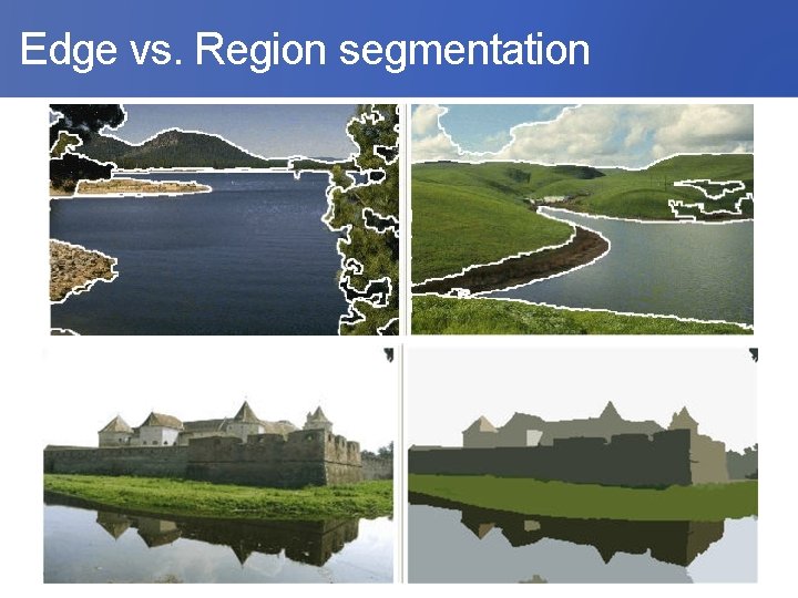
Edge vs. Region segmentation

What is a region? • A group of pixels with similar properties. • Let define a region R of an image f as a connected homogenous subset of the image with respect to some criterion. • The criterion makes pixels that correspond to each other to be grouped together / marked. • Some possible criterions are: gray value difference , gray value variance, Euclidean distance and so on.

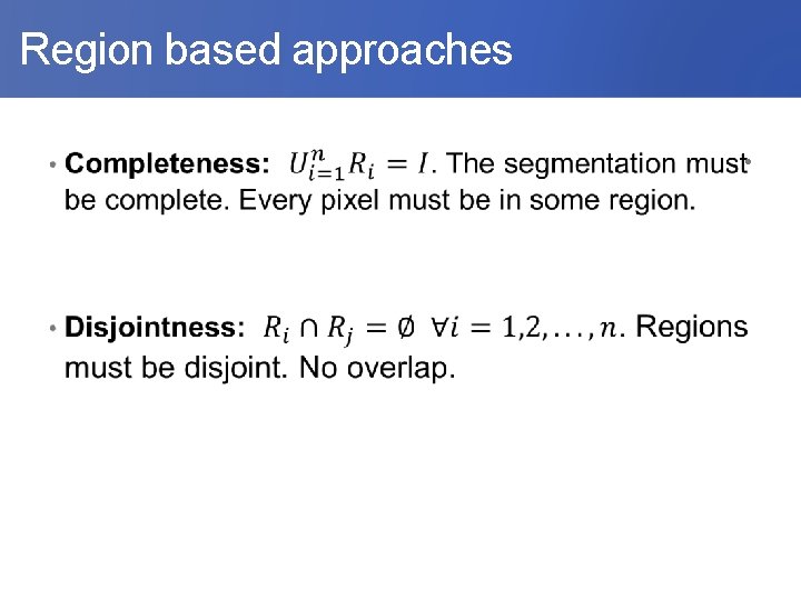
Region based approaches •

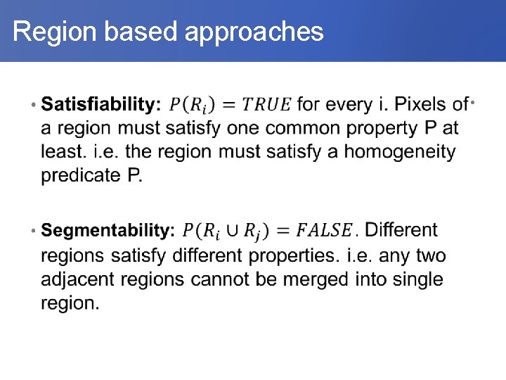
Region based approaches •

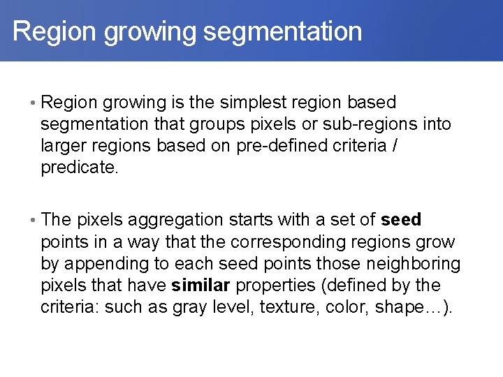
Region growing segmentation • Region growing is the simplest region based segmentation that groups pixels or sub-regions into larger regions based on pre-defined criteria / predicate. • The pixels aggregation starts with a set of seed points in a way that the corresponding regions grow by appending to each seed points those neighboring pixels that have similar properties (defined by the criteria: such as gray level, texture, color, shape…).

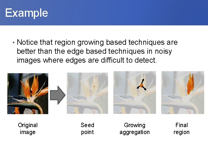
Example • Notice that region growing based techniques are better than the edge based techniques in noisy images where edges are difficult to detect. Original image Seed point Growing aggregation Final region

Seed based region growing segmentation • Pseudocode: • Let R be a region to extract. • Initially, the region R only contains its seed point p. • Let F be a FIFO queue that contains the boundary points of R. • Initially, F contains the 8 -neighborhood of the seed point p.

Seed based region growing segmentation • While F is not empty • For each neighbor pixel p* of p in F • If p* is similar to p • p* is added to R • Neighbor pixels of p* (not in R) are added to F. • Else • Set p* as non-similar (a new seed point).

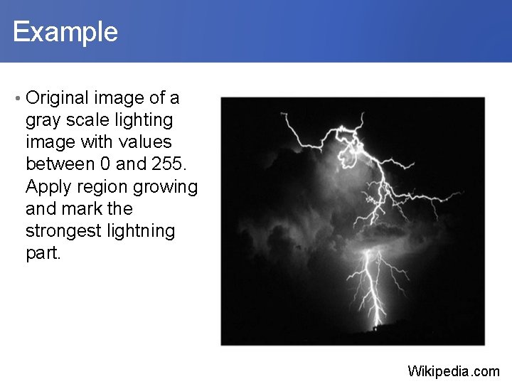
Example • Original image of a gray scale lighting image with values between 0 and 255. Apply region growing and mark the strongest lightning part. Wikipedia. com

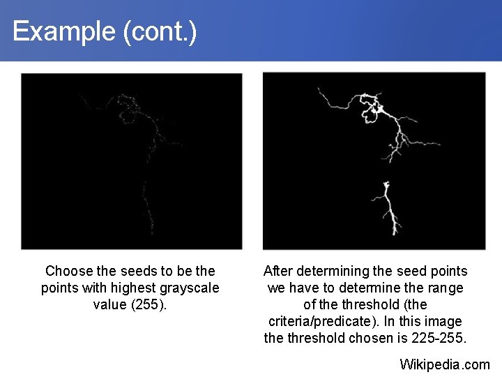
Example (cont. ) Choose the seeds to be the points with highest grayscale value (255). After determining the seed points we have to determine the range of the threshold (the criteria/predicate). In this image threshold chosen is 225 -255. Wikipedia. com

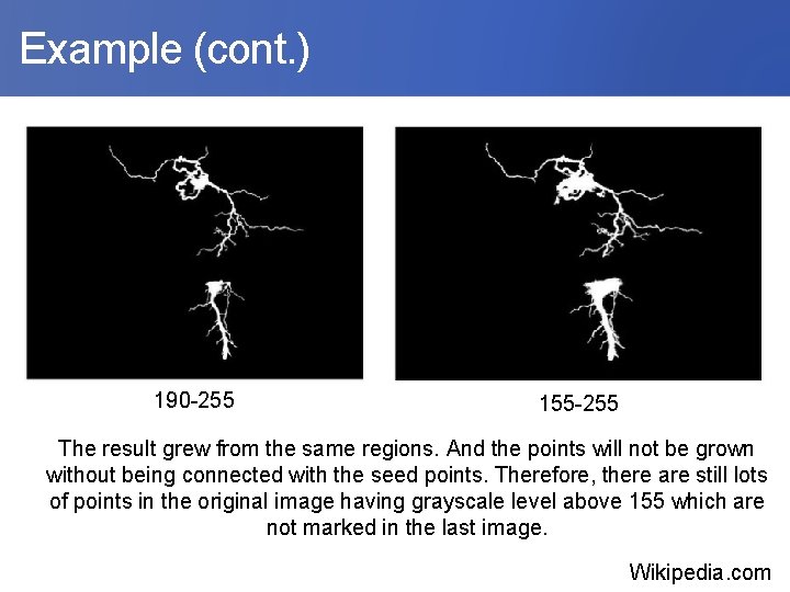
Example (cont. ) 190 -255 155 -255 The result grew from the same regions. And the points will not be grown without being connected with the seed points. Therefore, there are still lots of points in the original image having grayscale level above 155 which are not marked in the last image. Wikipedia. com

Advantages and disadvantages • Region growing methods can correctly separate the regions that have the same properties we define. • The concept is simple and fast. We only need a small number of seed points to represent the property we want and then grow the region. • The method is local. We have no global view of the problem. • So lets view another tool for segmentation.

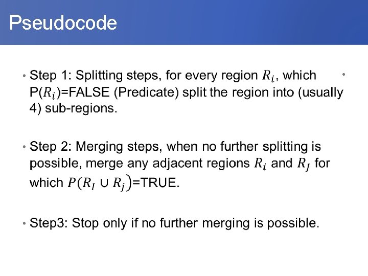
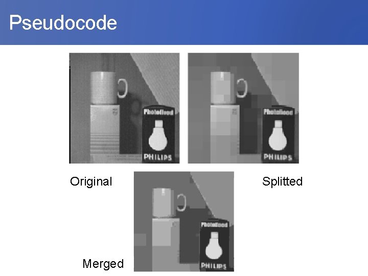
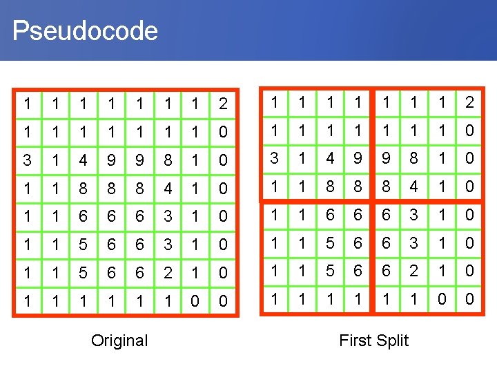
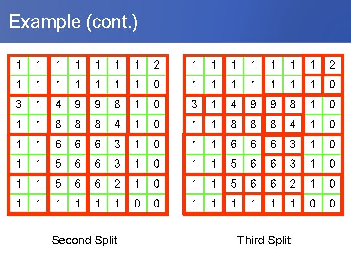
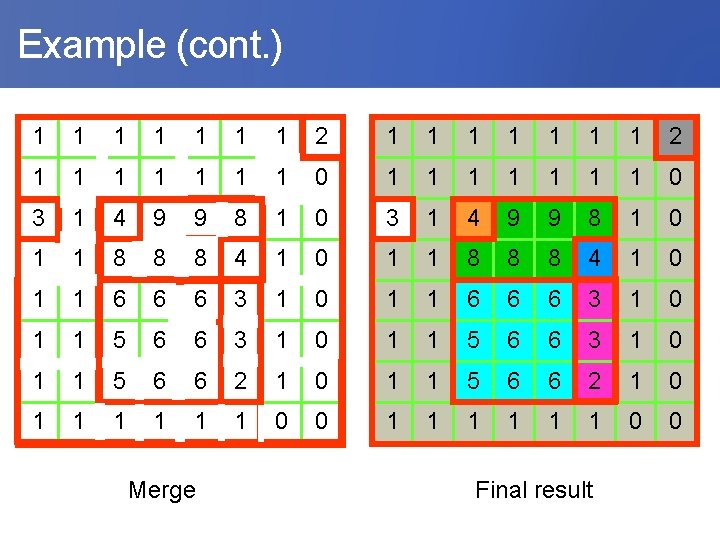
Region splitting and merging segmentation • Unlike region growing which starts from a set of seed points, region splitting starts with the whole image as a single region and subdivides it into sub-regions recursively while a condition of homogeneity is not satisfied. • Region merging is the opposite of region splitting and is being used to avoid over segmentation.

Pseudocode •

Pseudocode Original Merged Splitted

Pseudocode 1 1 1 1 2 1 1 1 1 0 3 1 4 9 9 8 1 0 1 1 8 8 8 4 1 0 1 1 6 6 6 3 1 0 1 1 5 6 6 2 1 0 1 1 1 0 0 Original First Split

Example (cont. ) 1 1 1 1 2 1 1 1 1 0 3 1 4 9 9 8 1 0 1 1 8 8 8 4 1 0 1 1 6 6 6 3 1 0 1 1 5 6 6 2 1 0 1 1 1 0 0 Second Split Third Split

Example (cont. ) 1 1 1 1 2 1 1 1 1 0 3 1 4 9 9 8 1 0 1 1 8 8 8 4 1 0 1 1 6 6 6 3 1 0 1 1 5 6 6 2 1 0 1 1 1 0 0 Merge Final result

Split and merge criterias •

Example Original

Example Original

Example Original

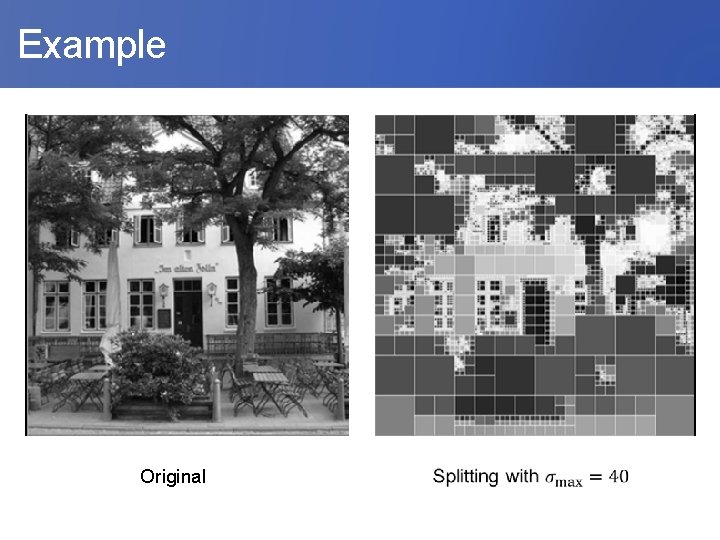
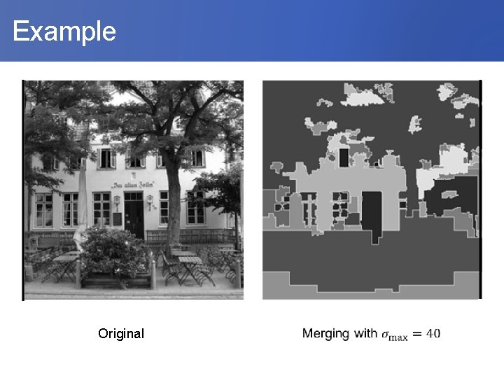
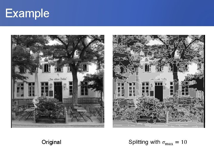
Advantages • The image could be split progressively according to our demanded resolution because the number of splitting level is determined by us. • We could split the image using the criteria we decide, such as mean or variance of segment pixel value. In addition, the merging criteria could be different to the splitting criteria.

Disadvantages • It may produce the “blocky” segments. This problem could be reduced by splitting in higher level, but the trade off is that computation time will arise. • A partially processed image would not contain a few clear, dominant regions in the image, but would contain many small unmerged regions.

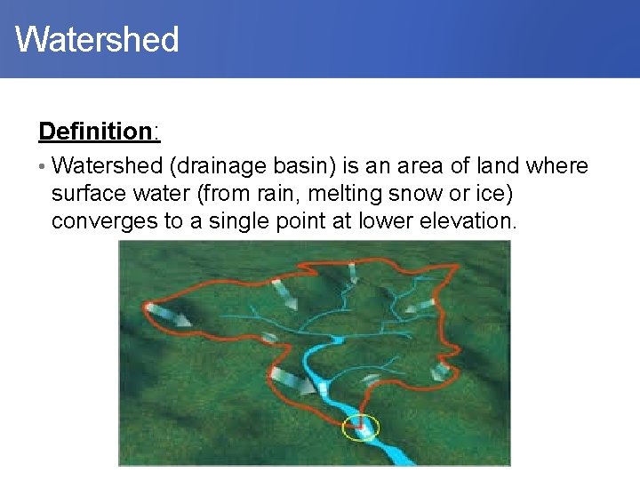
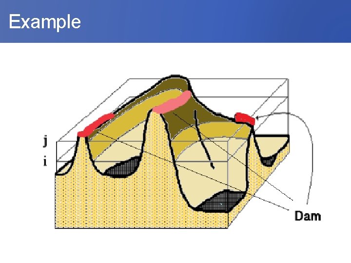
Watershed Definition: • Watershed (drainage basin) is an area of land where surface water (from rain, melting snow or ice) converges to a single point at lower elevation.

Watershed transformation • The intuitive idea underlying this method comes from geography. • Watershed transformation belongs to the region- based approach. • Will be talking about the concept introduced by Beucher S. and Lantuejoul C. (1979).

Example

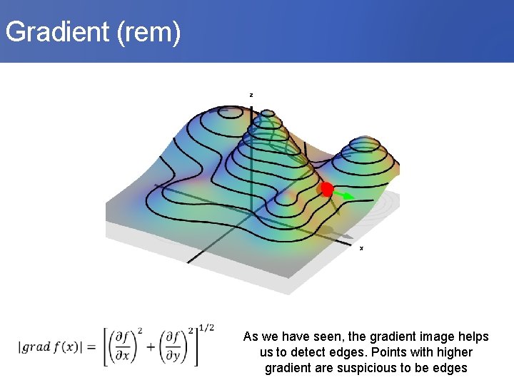
Gradient (rem) As we have seen, the gradient image helps us to detect edges. Points with higher gradient are suspicious to be edges

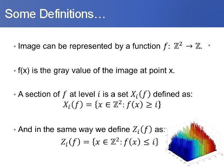
Some Definitions… •

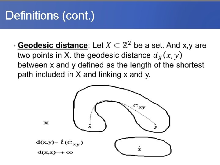
Definitions (cont. ) •

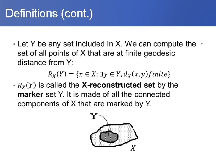
Definitions (cont. ) •

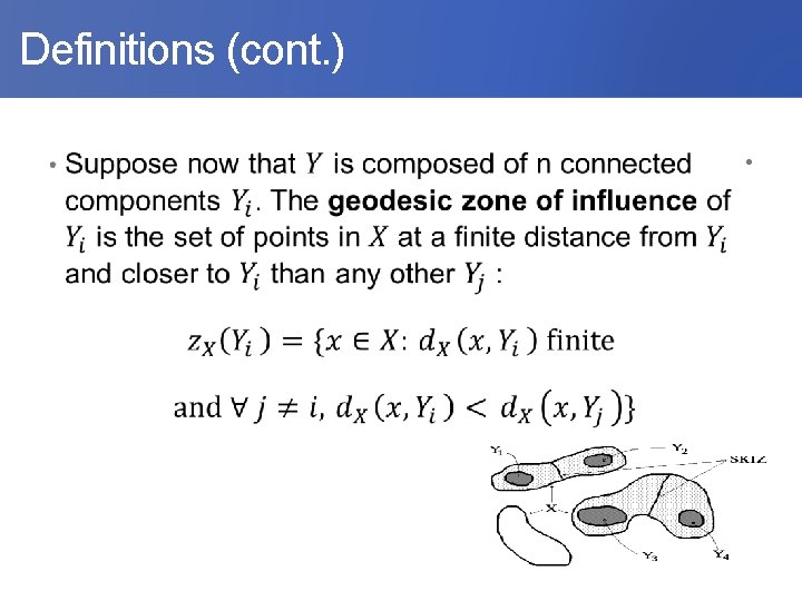
Definitions (cont. ) •

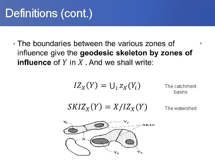
Definitions (cont. ) • The catchment basins The watershed

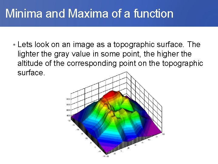
Minima and Maxima of a function • Lets look on an image as a topographic surface. The lighter the gray value in some point, the higher the altitude of the corresponding point on the topographic surface.

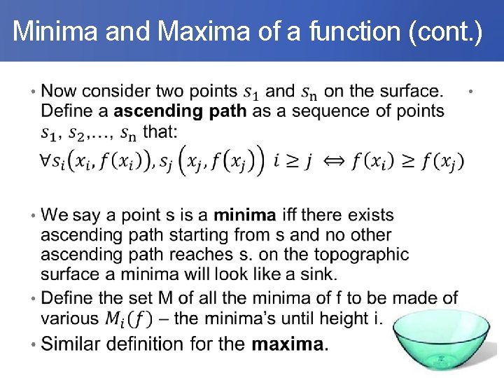
Minima and Maxima of a function (cont. ) •

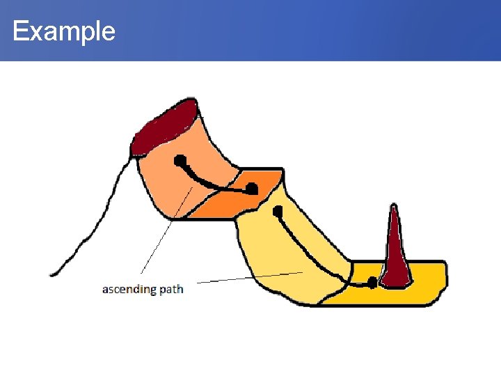
Example

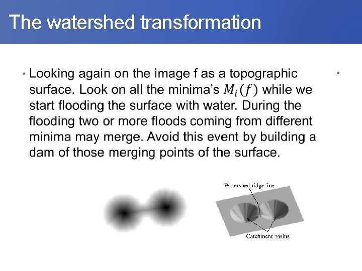
The watershed transformation •

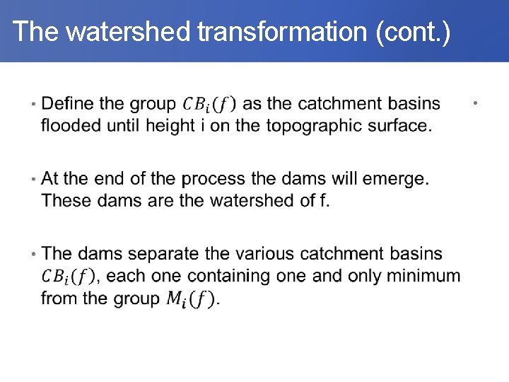
The watershed transformation (cont. ) •

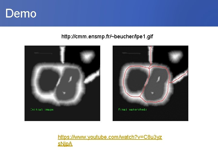
Demo http: //cmm. ensmp. fr/~beucher/lpe 1. gif https: //www. youtube. com/watch? v=C 8 u 3 yz s. Njp. A

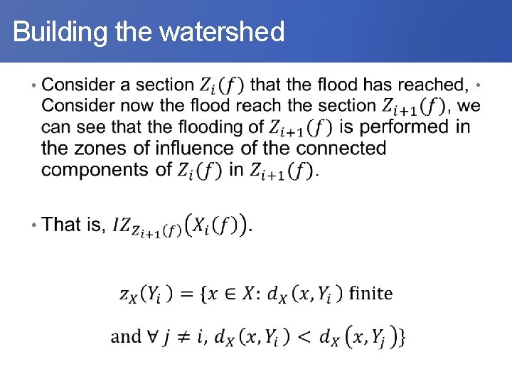
Building the watershed •

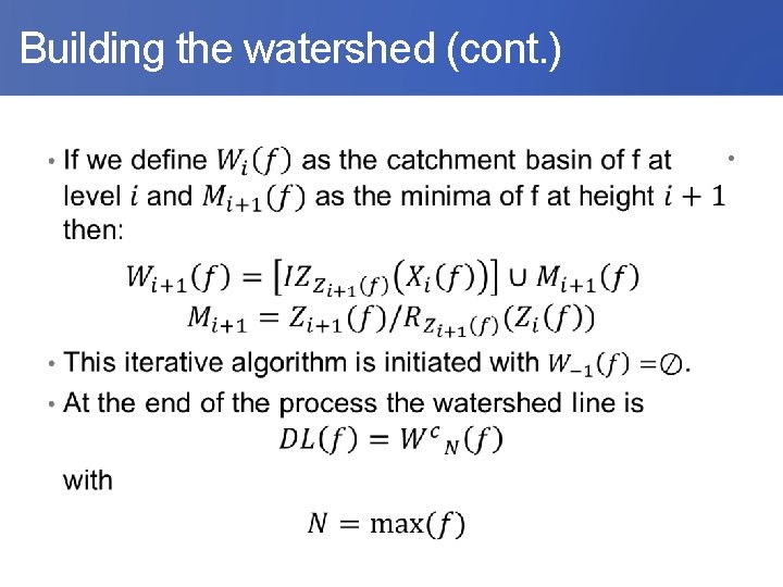
Building the watershed (cont. ) •

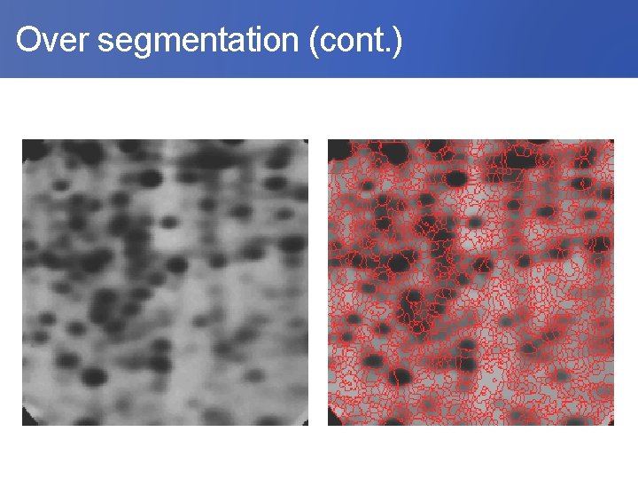
Over segmentation • Unfortunately using watershed transform on some of the gradient images we may get to much catchment basins. • Each one of them corresponds to a minimum of the gradient. • These minima are produced by small variations mainly due to image noise in the gray values.

Over segmentation (cont. )

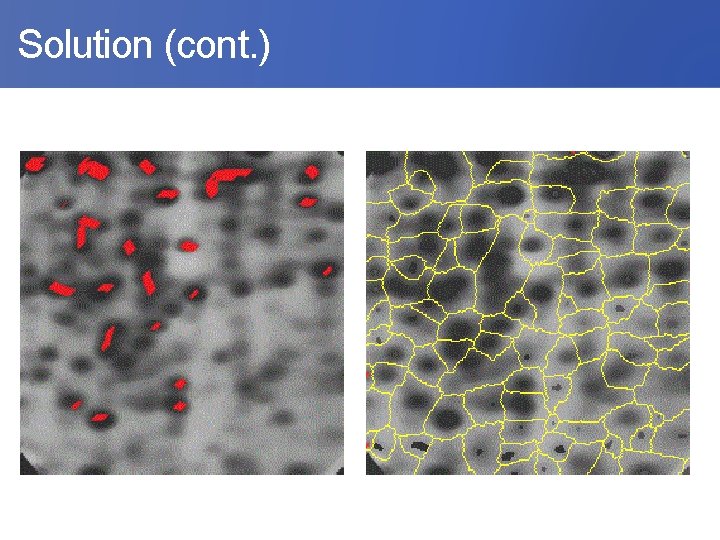
Solution • Mark the patterns to be segmented before performing the watershed transform. • And now instead of taking the whole image M set of minima’s we will start the algorithm on the minima’s at the markers patterns we chose.

Solution (cont. )

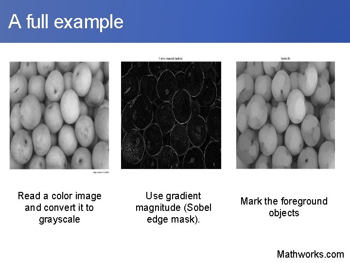
A full example Read a color image and convert it to grayscale Use gradient magnitude (Sobel edge mask). Mark the foreground objects Mathworks. com

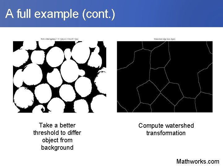
A full example (cont. ) Take a better threshold to differ object from background Compute watershed transformation Mathworks. com

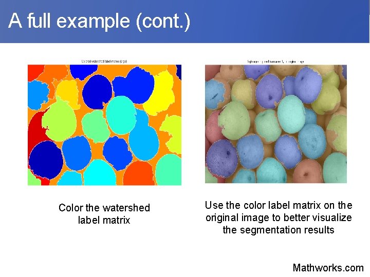
A full example (cont. ) Color the watershed label matrix Use the color label matrix on the original image to better visualize the segmentation results Mathworks. com

Another algorithm • The watershed algorithms can be divided in two groups. • The first group contains algorithms which simulate the flooding process. The second group is made of procedures aiming at the direct detection of the watershed points. • The algorithm we saw belongs to the first group. It simulates the flooding of the surface S starting from the minima of f.

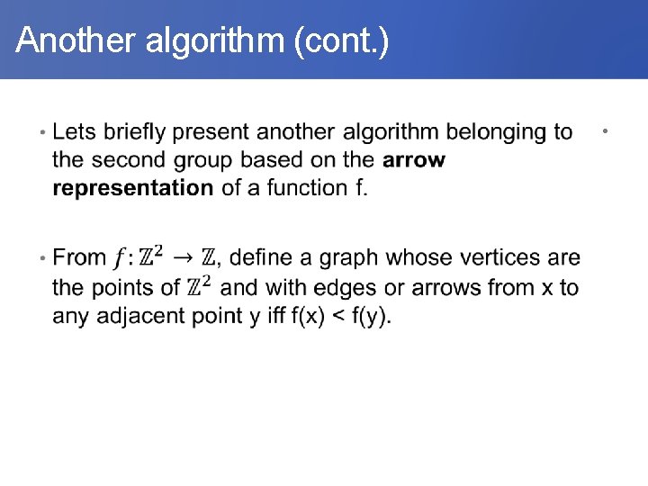
Another algorithm (cont. ) •

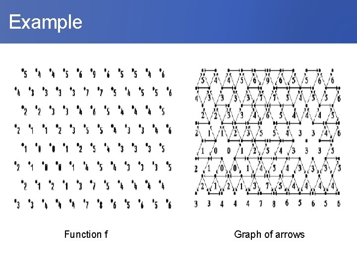
Example Function f Graph of arrows

Another algorithm (cont. ) • The definition of this graph does not allow the arrowing of the plateaus of the topographic surface. • Any point receiving arrows from more than one connected component of its neighborhood may be flooded by different lakes. Consequently, this point will be treated as a watershed and a dam will be built. • Doing so , we will change the arrowing of the neighborhood points and consequently the graph of arrows.

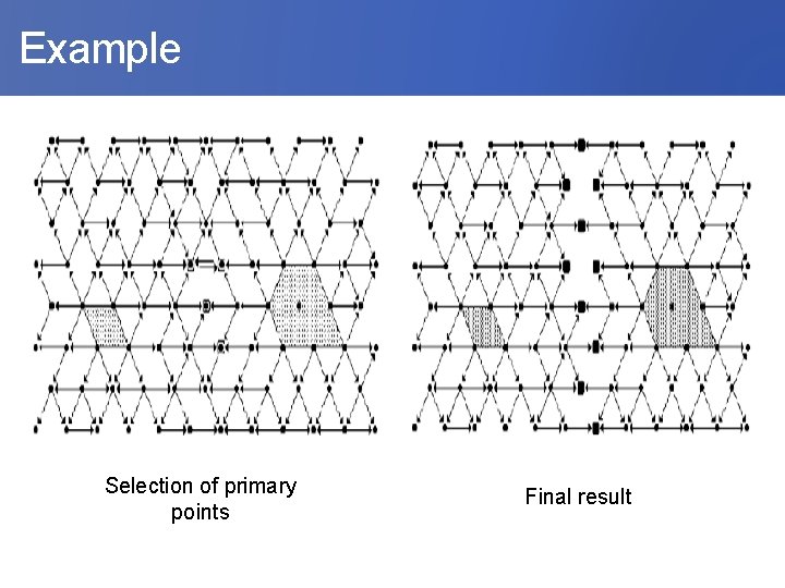
Example Selection of primary points Final result

Another algorithm (cont. ) • This procedure of selecting points can be re-run on each graph that we build so more divide may appear. • Re-run the procedure until no new divide points is selected. • The algorithm produces local watershed lines. The true divide lines will be extracted easily but the divide points with smaller curves will be harder to detect.

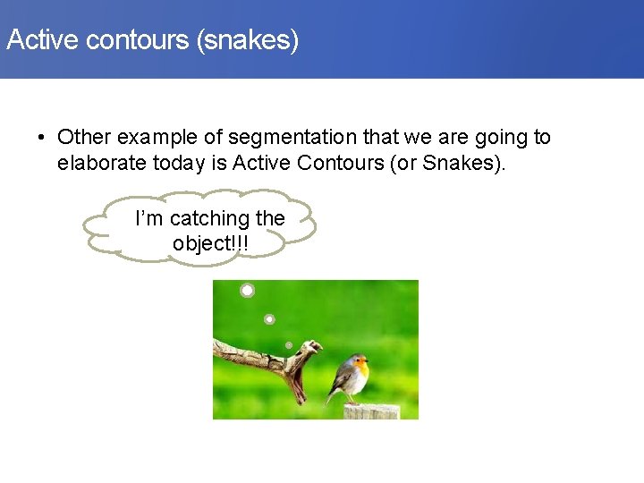
Active contours (snakes) • Other example of segmentation that we are going to elaborate today is Active Contours (or Snakes). I’m catching the object!!!

History • A framework in Computer vision and image processing. • Appeared in the first ICCV conference in 1987. • Michael Kass, Andrew Witkin, and Demetri Terzopoulos.

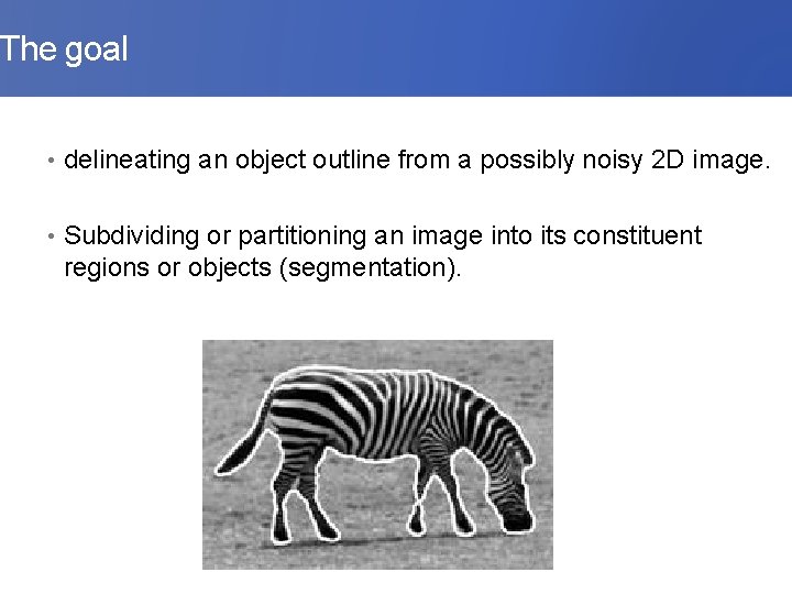
The goal • delineating an object outline from a possibly noisy 2 D image. • Subdividing or partitioning an image into its constituent regions or objects (segmentation).

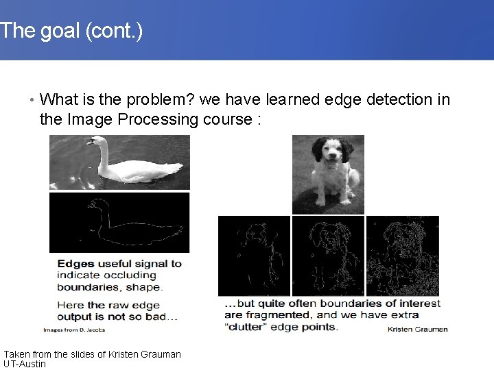
The goal (cont. ) • What is the problem? we have learned edge detection in the Image Processing course : Taken from the slides of Kristen Grauman UT-Austin

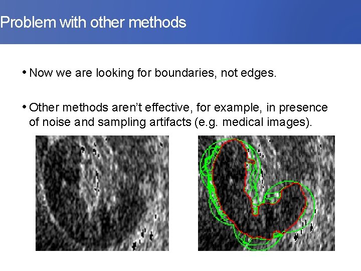
Problem with other methods • Now we are looking for boundaries, not edges. • Other methods aren’t effective, for example, in presence of noise and sampling artifacts (e. g. medical images).

What is snake? • A snake is deformable spline influenced by constraint and image forces that pull it towards object contours and internal forces that resist deformation (internal and external energies). • They autonomously and adaptively search for the minimum state. • They can be used to track dynamic objects.

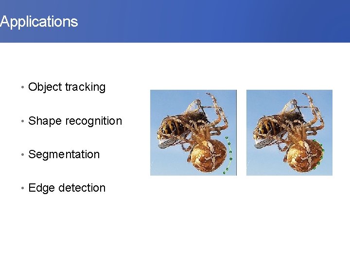
Applications • Object tracking • Shape recognition • Segmentation • Edge detection

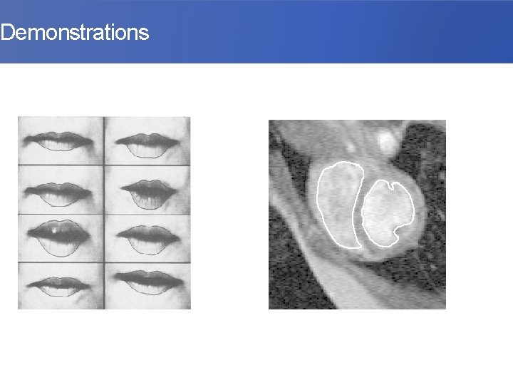
Demonstrations

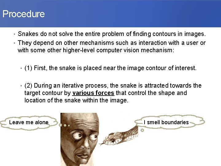
Procedure • Snakes do not solve the entire problem of finding contours in images. • They depend on other mechanisms such as interaction with a user or with some other higher-level computer vision mechanism: • (1) First, the snake is placed near the image contour of interest. • (2) During an iterative process, the snake is attracted towards the target contour by various forces that control the shape and location of the snake within the image. Leave me alone I smell boundaries

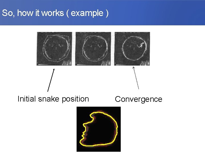
So, how it works ( example ) Initial snake position Convergence

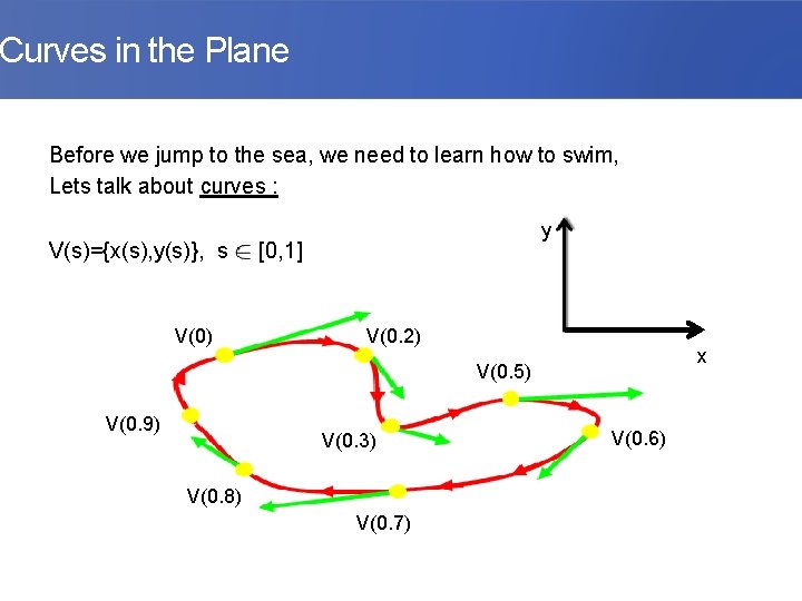
Curves in the Plane Before we jump to the sea, we need to learn how to swim, Lets talk about curves : y V(s)={x(s), y(s)}, s [0, 1] V(0) V(0. 2) x V(0. 5) V(0. 9) V(0. 3) V(0. 8) V(0. 7) V(0. 6)

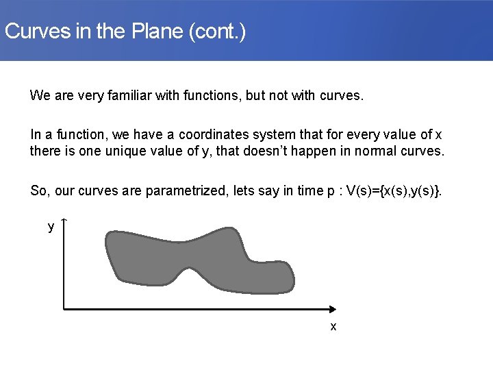
Curves in the Plane (cont. ) We are very familiar with functions, but not with curves. In a function, we have a coordinates system that for every value of x there is one unique value of y, that doesn’t happen in normal curves. So, our curves are parametrized, lets say in time p : V(s)={x(s), y(s)}. y x

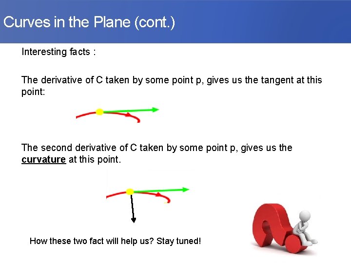
Curves in the Plane (cont. ) Interesting facts : The derivative of C taken by some point p, gives us the tangent at this point: The second derivative of C taken by some point p, gives us the curvature at this point. How these two fact will help us? Stay tuned!

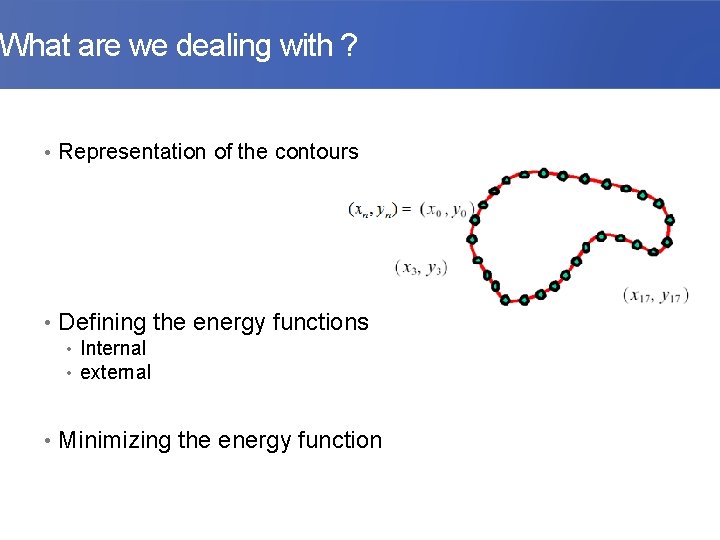
What are we dealing with ? • Representation of the contours • Defining the energy functions • Internal • external • Minimizing the energy function

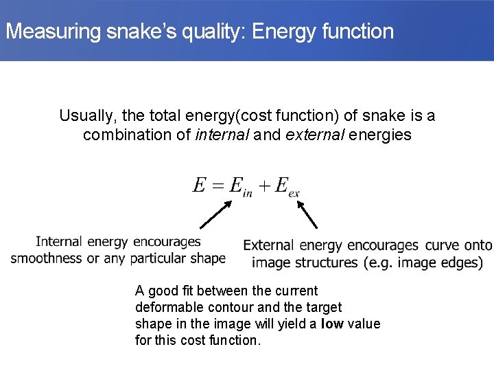
Measuring snake’s quality: Energy function Usually, the total energy(cost function) of snake is a combination of internal and external energies A good fit between the current deformable contour and the target shape in the image will yield a low value for this cost function.

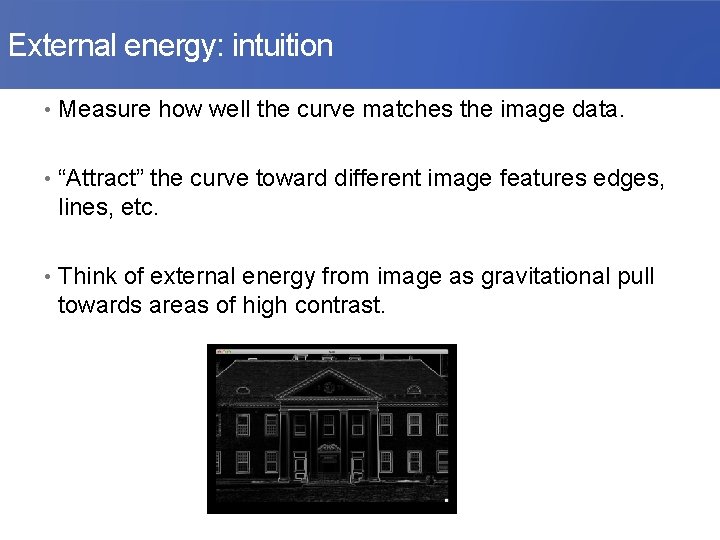
External energy: intuition • Measure how well the curve matches the image data. • “Attract” the curve toward different image features edges, lines, etc. • Think of external energy from image as gravitational pull towards areas of high contrast.

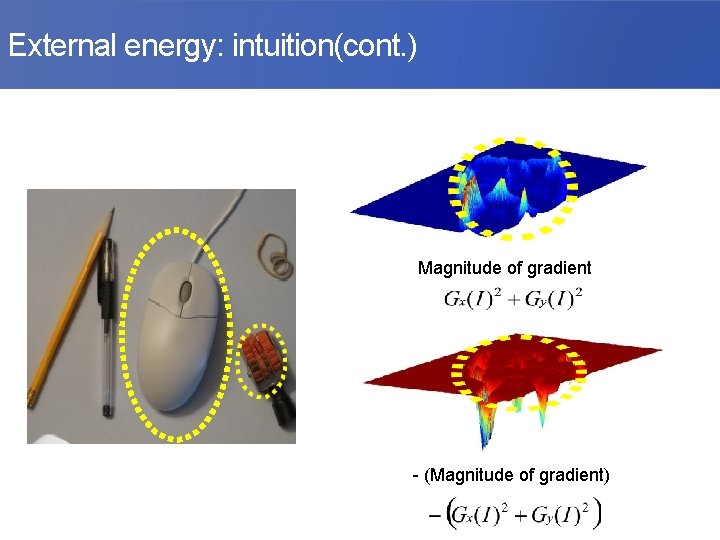
External energy: intuition(cont. ) Magnitude of gradient - (Magnitude of gradient)

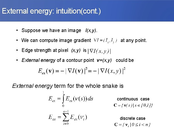
External energy: intuition(cont. ) • Suppose we have an image I(x, y). • We can compute image gradient at any point. • Edge strength at pixel (x, y) is • External energy of a contour point v=(x, y) could be External energy term for the whole snake is continuous case discrete case

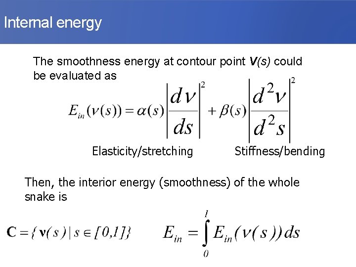
Internal energy The smoothness energy at contour point V(s) could be evaluated as Elasticity/stretching Stiffness/bending Then, the interior energy (smoothness) of the whole snake is

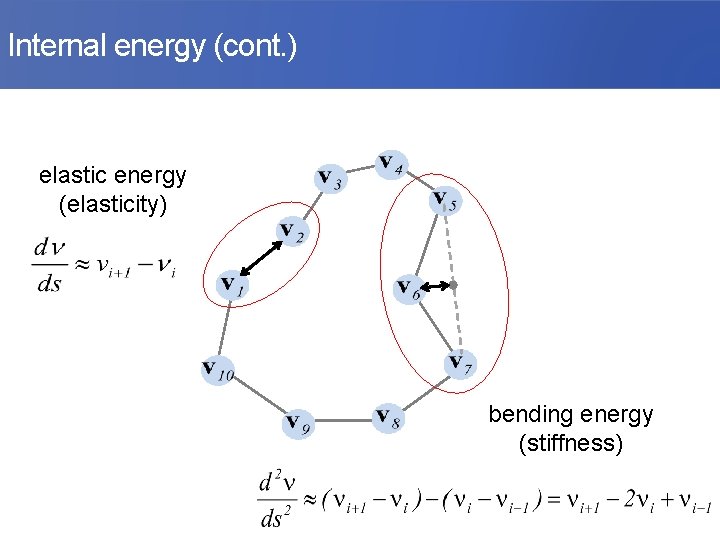
Internal energy (cont. ) elastic energy (elasticity) bending energy (stiffness)

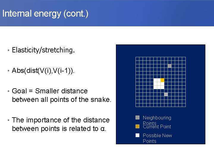
Internal energy (cont. ) • Elasticity/stretching. • Abs(dist(V(i), V(i-1)). • Goal = Smaller distance between all points of the snake. • The importance of the distance between points is related to α. Neighbouring Points Current Point Possible New Points

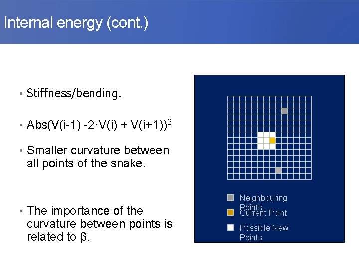
Internal energy (cont. ) • Stiffness/bending. • Abs(V(i-1) -2·V(i) + V(i+1))2 • Smaller curvature between all points of the snake. • The importance of the curvature between points is related to β. Neighbouring Points Current Point Possible New Points

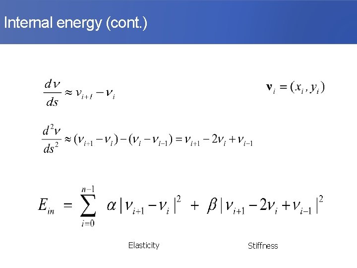
Internal energy (cont. ) Elasticity Stiffness

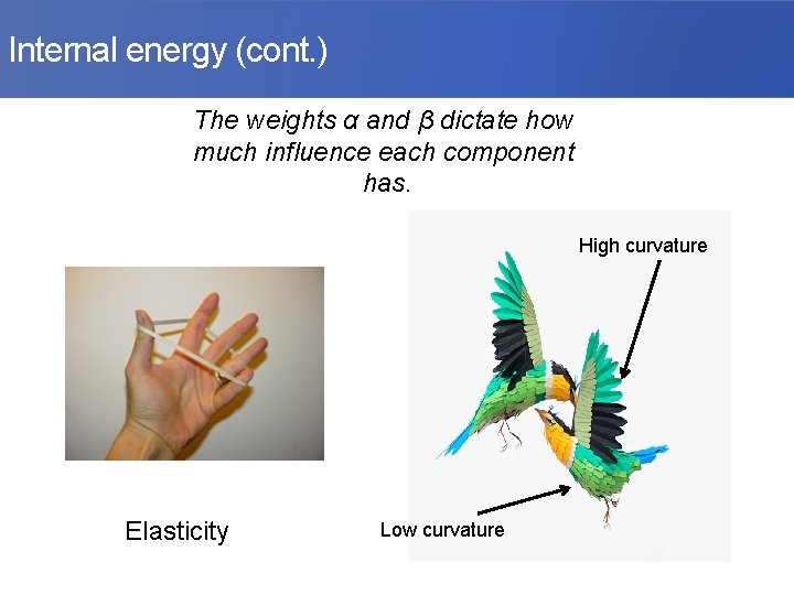
Internal energy (cont. ) The weights α and β dictate how much influence each component has. High curvature Elasticity Low curvature

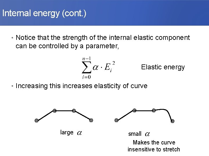
Internal energy (cont. ) • Notice that the strength of the internal elastic component can be controlled by a parameter, Elastic energy • Increasing this increases elasticity of curve large small Makes the curve insensitive to stretch

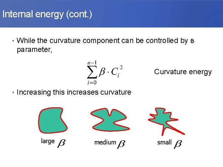
Internal energy (cont. ) • While the curvature component can be controlled by ʙ parameter, Curvature energy • Increasing this increases curvature large medium small

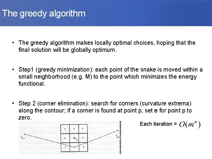
The greedy algorithm • The greedy algorithm makes locally optimal choices, hoping that the final solution will be globally optimum. • Step 1 (greedy minimization): each point of the snake is moved within a small neighborhood (e. g. M) to the point which minimizes the energy functional. • Step 2 (corner elimination): search for corners (curvature extrema) along the contour; if a corner is found at point p, set ʙ for point p to zero. Each iteration =

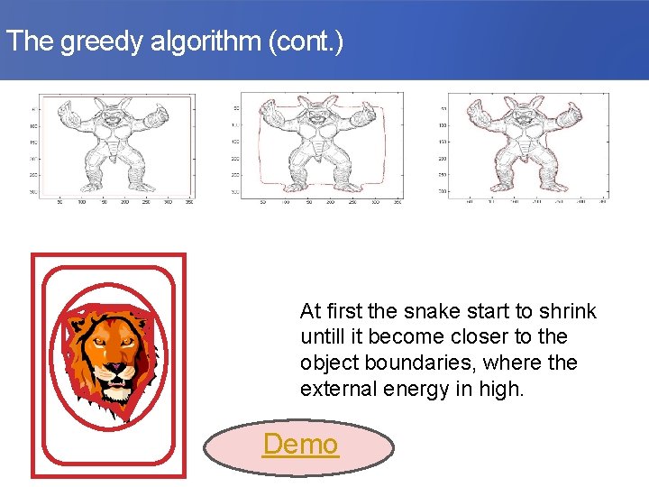
The greedy algorithm (cont. ) At first the snake start to shrink untill it become closer to the object boundaries, where the external energy in high. Demo

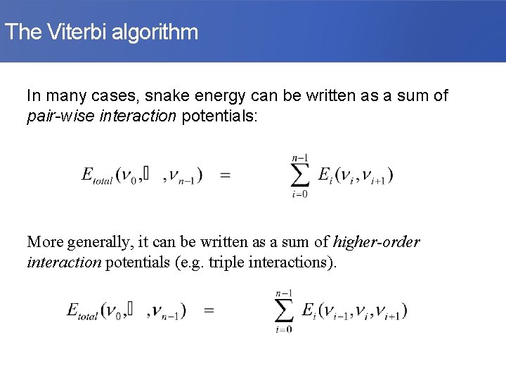
The Viterbi algorithm In many cases, snake energy can be written as a sum of pair-wise interaction potentials: More generally, it can be written as a sum of higher-order interaction potentials (e. g. triple interactions).

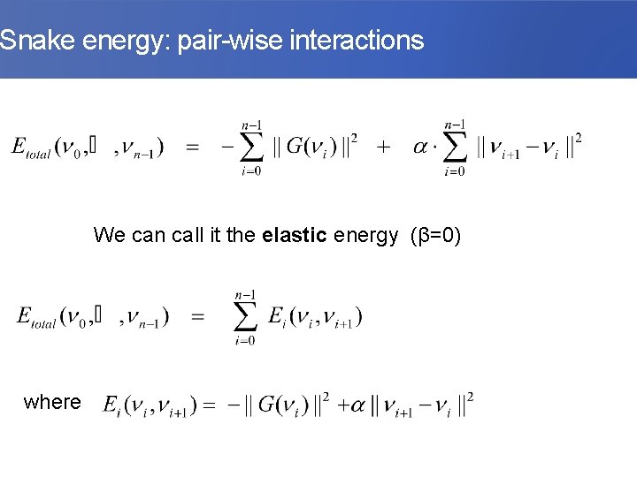
Snake energy: pair-wise interactions We can call it the elastic energy (β=0) where

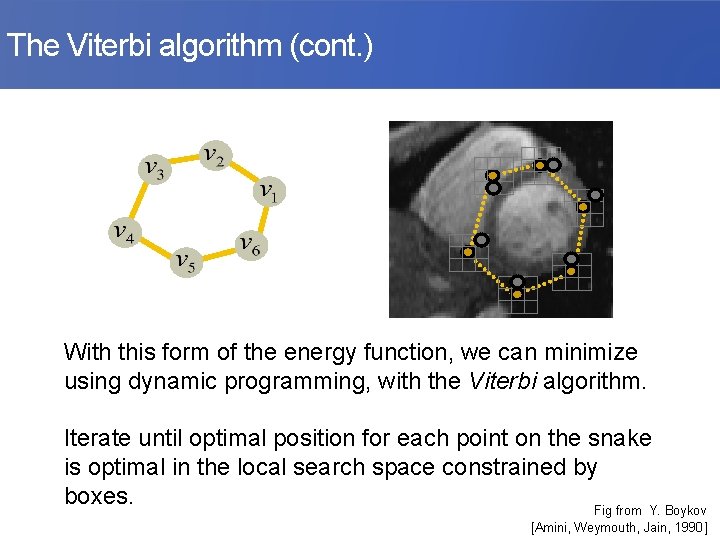
The Viterbi algorithm (cont. ) With this form of the energy function, we can minimize using dynamic programming, with the Viterbi algorithm. Iterate until optimal position for each point on the snake is optimal in the local search space constrained by boxes. Fig from Y. Boykov [Amini, Weymouth, Jain, 1990]

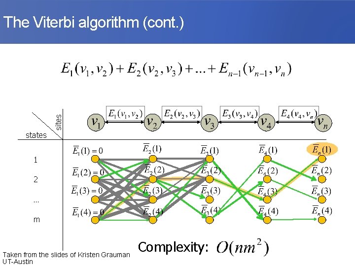
5 -91 states sites The Viterbi algorithm (cont. ) 1 2 … m Taken from the slides of Kristen Grauman UT-Austin Complexity:

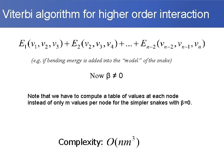
Viterbi algorithm for higher order interaction (e. g. if bending energy is added into the “model” of the snake) Now β ≠ 0 Note that we have to compute a table of values at each node instead of only m values per node for the simpler snakes with β=0. Complexity:

Extensions • What if the input curve starts inside the object we are looking for? . • What happens if we have multiple object we want to detect? .

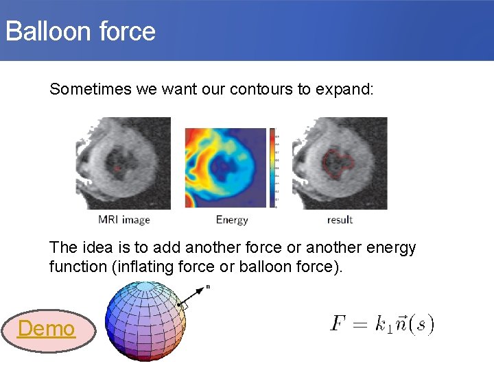
Balloon force Sometimes we want our contours to expand: The idea is to add another force or another energy function (inflating force or balloon force). Demo

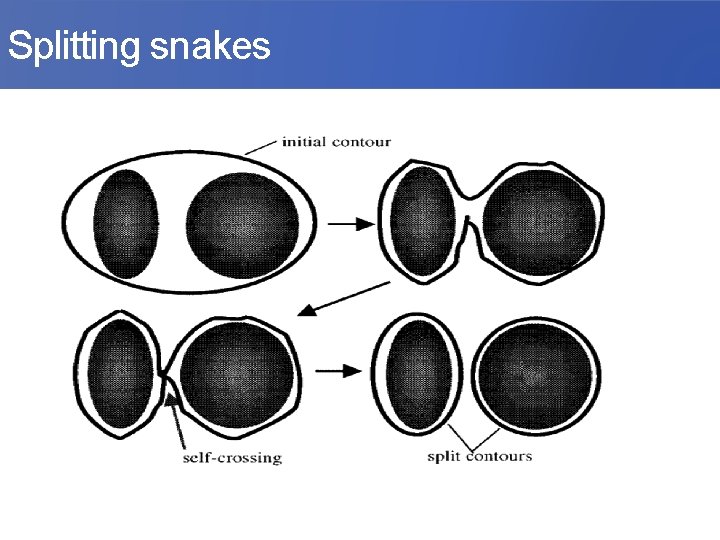
Splitting snakes

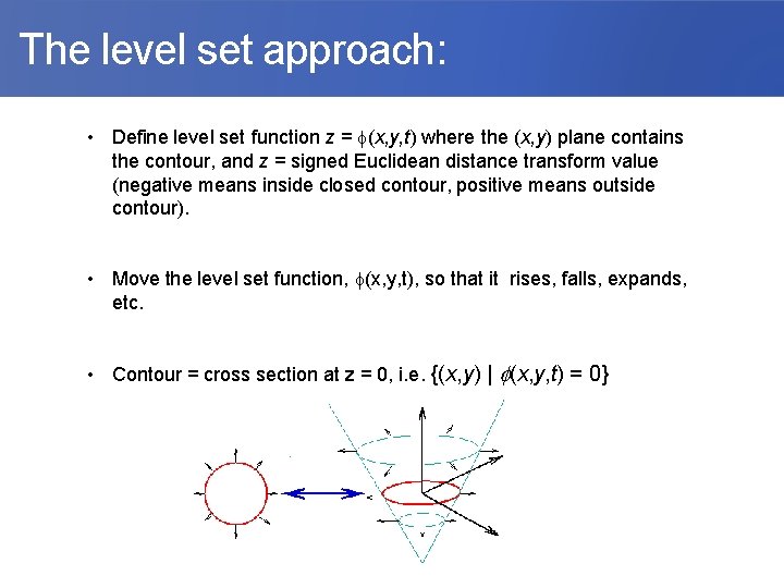
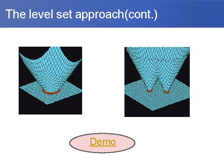
The level set approach: • Define level set function z = (x, y, t) where the (x, y) plane contains the contour, and z = signed Euclidean distance transform value (negative means inside closed contour, positive means outside contour). • Move the level set function, (x, y, t), so that it rises, falls, expands, etc. • Contour = cross section at z = 0, i. e. {(x, y) | (x, y, t) = 0}

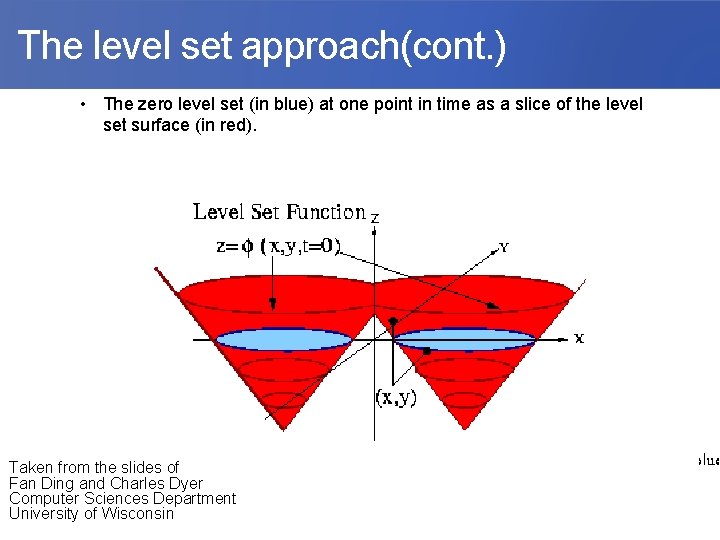
The level set approach(cont. ) • The zero level set (in blue) at one point in time as a slice of the level set surface (in red). Taken from the slides of Fan Ding and Charles Dyer Computer Sciences Department University of Wisconsin

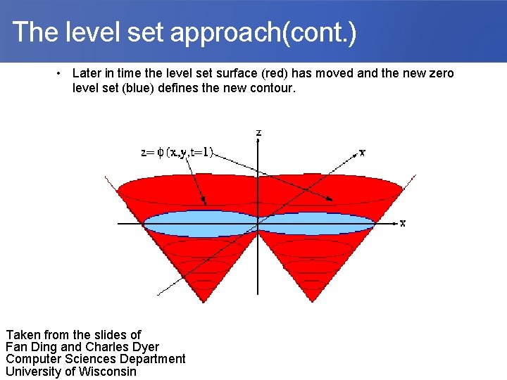
The level set approach(cont. ) • Later in time the level set surface (red) has moved and the new zero level set (blue) defines the new contour. Taken from the slides of Fan Ding and Charles Dyer Computer Sciences Department University of Wisconsin

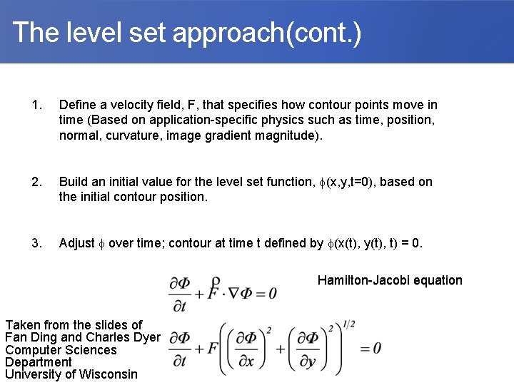
The level set approach(cont. ) 1. Define a velocity field, F, that specifies how contour points move in time (Based on application-specific physics such as time, position, normal, curvature, image gradient magnitude). 2. Build an initial value for the level set function, (x, y, t=0), based on the initial contour position. 3. Adjust over time; contour at time t defined by (x(t), y(t), t) = 0. Hamilton-Jacobi equation Taken from the slides of Fan Ding and Charles Dyer Computer Sciences Department University of Wisconsin

The level set approach(cont. ) Demo

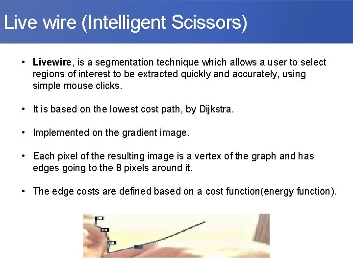
Live wire (Intelligent Scissors) • Livewire, is a segmentation technique which allows a user to select regions of interest to be extracted quickly and accurately, using simple mouse clicks. • It is based on the lowest cost path, by Dijkstra. • Implemented on the gradient image. • Each pixel of the resulting image is a vertex of the graph and has edges going to the 8 pixels around it. • The edge costs are defined based on a cost function(energy function).

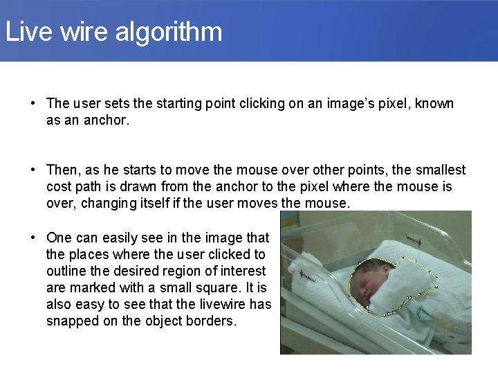
Live wire algorithm • The user sets the starting point clicking on an image’s pixel, known as an anchor. • Then, as he starts to move the mouse over other points, the smallest cost path is drawn from the anchor to the pixel where the mouse is over, changing itself if the user moves the mouse. • One can easily see in the image that the places where the user clicked to outline the desired region of interest are marked with a small square. It is also easy to see that the livewire has snapped on the object borders.

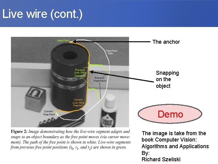
Live wire (cont. ) The anchor Snapping on the object Demo The image is take from the book Computer Vision: Algorithms and Applications By: Richard Szeliski

Summary • Segmentation: essential first step in the most scenes of analysis and recognition problems of images. • A universal algorithm of segmentation doesn’t exist, as each type of image corresponds of a specific approach. • Applications: finding tumors, veins etc. in medical images, finding targets in satellite/aerial images, finding people in surveillance images, snakes, scissors etc.

References • Region based segmentation: Marc Polmlun http: //www. cs. umb. edu/~marc/cs 675/cpv 10 -28. pdf • Split and Merge tutorial: (CV-online) http: //homepages. inf. ed. ac. uk/rbf/CVonline/LOCAL_COPIES/MARBL E/medium/segment/split. htm • Watershed-Based Segmentation and Region Merging Andre bleau, L. joshua Leon. http: //www. sciencedirect. com/science/article/pii/S 1077314299908226 Michael Kass, Andrew Witkin, Demetri Terzopoulos. • http: //link. springer. com/article/10. 1007/BF 00133570#page-1 • http: //link. springer. com/article/10. 1023/A: 1007922224810#page-1 • http: //en. wikipedia. org/wiki/Image_segmentation

References George Bebis http: //www. cse. unr. edu/~bebis/CS 791 E/Notes/Def ormable. Contours. pdf Kristen Grauman. http: //www. cs. utexas. edu/~grauman/courses/378/ handouts/snakes. pdf Jana Kosecka http: //cs. gmu. edu/~kosecka/cs 682/lect-snakes. pdf