Section 9 2 Inferences About Two Proportions Copyright

Review • In Chapters 7 and 8 we introduced methods of inferential statistics. • In Chapter 7 we presented methods of constructing confidence interval estimates of population parameters. • In Chapter 8 we presented methods of testing claims made about population parameters. • Chapters 7 and 8 both involved methods for dealing with a sample from a single population.

Preview �Test the claim that when college students are weighed at the beginning and end of their freshman year, the differences show a mean weight gain of 15 pounds (as in the “Freshman 15” belief). �Test the claim that the proportion of children who contract polio is less for children given the Salk vaccine than for children given a placebo. �Test the claim that subjects treated with Lipitor have a mean cholesterol level that is lower than the mean cholesterol level for subjects given a placebo.

Learning Targets In this section we present methods for (1) testing a claim made about the two population proportions and (2) constructing a confidence interval estimate of the difference between the two population proportions. This section is based on proportions, but we can use the same methods for dealing with probabilities or the decimal equivalents of percentages.

Notation for Two Proportions For population 1, we let: p 1 = population proportion n 1 = size of the sample x 1 = number of successes in the sample x 1 ^ p = n (the sample proportion) 1 1 q^1 = 1 – p^1 The corresponding notations apply to p , n , x , p^. and q^ , which come from population 2. 2 2 2

Pooled Sample Proportion v The pooled sample proportion is denoted by p and is given by: x 1 + x 2 p= n +n 1 2 v We denote the complement of p by q, so q = 1–p

Requirements 1. We have proportions from two independent simple random samples. 2. For each of the two samples, the number of successes is at least 5 and the number of failures is at least 5.

Test Statistic for Two Proportions For H 0: p 1 = p 2 H 1: p 1 p 2 , z= H 1: p 1 < p 2 , H 1: p 1> p 2 ^ )–(p –p ) ( p^1 – p 2 1 2 pq pq + n 2 n 1 = ( p^1 – p^2 ) pq (n 1 1 + n 2 where p – p = 0 (assumed in the null hypothesis) 1 2 1 )

Test Statistic for Two Proportions – Cont… Critical values: Use inv. Norm(area to the left, 0, 1) *left tailed test, α is in the left tail *right tailed test, α is in the right tail *two tailed test, α is divided equally between the two tails. P-values: Use the normalcdf feature on your calculator Right-tailed tests: To find this probability in your calculator, type: normalcdf (z test statistic, 99999, 0, 1) Left-tailed tests: To find this probability in your calculator, type: normalcdf (– 99999, –z test statistic, 0, 1) ***Don’t forget if your test is two-sided, double your P-value. ***

Example 1: The table below lists results from a simple random sample of front-seat occupants involved in car crashes. Use a 0. 05 significance level to test the claim that the fatality rate of occupants is lower for those in cars equipped with airbags. a) State the null hypothesis and the alternative hypothesis. H 0: p 1 = p 2 H 1: p 1 < p 2 b) Find the pooled estimate c) Find the critical value(s). inv. Norm(0. 05, 0, 1) = – 1. 645

d) Find the test statistic. e) Find the P-value = normalcdf(– 99999, – 1. 9116, 0 , 1) = 0. 0281 < 0. 05. Reject H 0. f) What is the conclusion? There is sufficient evidence to support the claim that the fatality rate of occupants is lower for those in cars equipped with airbags.

Example: Left-tailed test. Area to left of z = – 1. 9116 is 0. 0281 (Table A-2), so the P-value is 0. 0281. “STAT” “ 2 -Prop. ZTest” enter x 1=41, n 1 = 11541, x 2 = 52, n 2 = 9853 P-Value = 0. 0280

Example: Using the Traditional Method With a significance level of = 0. 05 in a left- tailed test based on the normal distribution, we refer to Table A-2 and find that an area of = 0. 05 in the left tail corresponds to the critical value of z = – 1. 645. The test statistic of does fall in the critical region bounded by the critical value of z = – 1. 645. We again reject the null hypothesis.

Caution When testing a claim about two population proportions, the P-value method and the traditional method are equivalent, but they are not equivalent to the confidence interval method. If you want to test a claim about two population proportions, use the P-value method or traditional method; if you want to estimate the difference between two population proportions, use a confidence interval.

Your Turn: A simple random sample of front-seat occupants involved in car crashes is obtained. Among 2823 occupants not wearing seat belts, 31 were killed. Among 7765 occupants wearing seat belts, 16 were killed (based on data from “Who Wants Airbags? ” by Meyer and Finney, Chance, Vol. 18, No. 2). Use a 0. 01 significance level to test the claim that the fatality rate is higher for those not wearing seat belts. a) State the null hypothesis and the alternative hypothesis. H 0: p 1 = p 2 H 1: p 1 > p 2 b) Find the pooled estimate c) Find the critical value(s). inv. Norm(1 – 0. 05, 0, 1) = 1. 6449

d) Find the test statistic. e) Find the P-value = normalcdf(6. 1058, 99999, 0, 1) ≈ 0 < 0. 01 Reject H 0. f) What is the conclusion? There is sufficient evidence to support the claim that the fatality rate is higher for those not wearing seat belts.

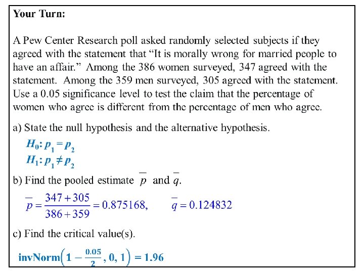
d) Find the test statistic. e) Find the p-value. P-value = 2 normalcdf(2. 0376, 99999, 0, 1) = 0. 02079 × 2 = 0. 04159 < 0. 05, Reject H 0. f) What is the conclusion? There is sufficient evidence to support that the percentage of women who agree is different from the percentage of men who agree.

Confidence Interval Estimate of p 1 – p 2 ( p^1 – p^2 ) – E < ( p 1 – p 2 ) < ( p^1 where E = z p^ q^ 1 n 1 1 + – p^2 ) + p^ q^ 2 n 2 2 E

Example: Use the sample data given in the preceding Example to construct a 90% confidence interval estimate of the difference between the two population proportions. (As shown in Table 8 -2 on page 406, the confidence level of 90% is comparable to the significance level of = 0. 05 used in the preceding left-tailed hypothesis test. ) What does the result suggest about the effectiveness of airbags in an accident?

Example: Requirements are satisfied as we saw in the preceding example. 90% confidence interval: z /2 = 1. 645 Calculate the margin of error, E

Example: Construct the confidence interval Short Cut: “STAT” “ 2 -Prop. ZInt” enter x 1=41, n 1 = 11541, x 2 = 52, n 2 = 9853 Confidence Interval (-0. 0032, -0. 0002).

Example: The confidence interval limits do not contain 0, implying that there is a significant difference between the two proportions. The confidence interval suggests that the fatality rate is lower for occupants in cars with air bags than for occupants in cars without air bags. The confidence interval also provides an estimate of the amount of the difference between the two fatality rates.

Example: A simple random sample of front-seat occupants involved in car crashes is obtained. Among 2823 occupants not wearing seat belts, 31 were killed. Among 7765 occupants wearing seat belts, 16 were killed (based on data from “Who Wants Airbags? ” by Meyer and Finney, Chance, Vol. 18, No. 2). Construct a 90% confidence interval estimate of the difference between the two population proportions. z* = inv. Norm(1 – 0. 05, 0, 1) = 1. 6449 Please remember that z* must be positive for confidence intervals!!!!! (0. 0089 – 0. 0033, 0. 0089 + 0. 0033) = (0. 0056, 0. 0123) This is your final answer!

Your Turn: A Pew Center Research poll asked randomly selected subjects if they agreed with the statement that “It is morally wrong for married people to have an affair. ” Among the 386 women surveyed, 347 agreed with the statement. Among the 359 men surveyed, 305 agreed with the statement. Construct a 95% confidence interval estimate of the difference between the two population proportions. z* = inv. Norm(0. 975, 0, 1) = 1. 96 Please remember that z* must be positive for confidence intervals!!!!! This is your final answer! (0. 0494 – 0. 0477, 0. 0494 + 0. 0477) = (0. 0017, 0. 0970)

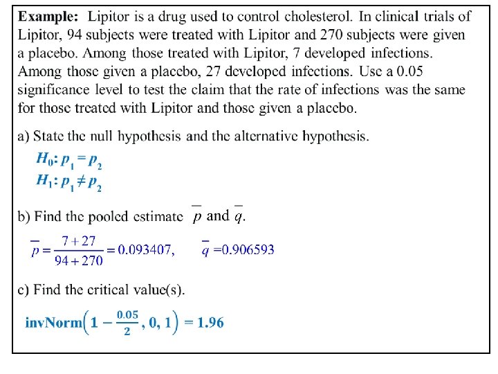
d) Find the test statistic. e) Find the P-value = 2 normalcdf(– 99999, – 0. 7326, 0, 1) = 2 × 0. 2319 = 0. 4638 > 0. 05, Fail to reject H 0. f) What is the conclusion? There is not sufficient evidence to support the claim that the rate of infections was not the same for those treated with Lipitor and those given a placebo.

g) Determine h) Find the margin of error. i) Construct a 95% confidence interval estimate of the difference between the two population proportions. (– 0. 0255 – 0. 064, – 0. 0255 + 0. 064) = (– 0. 0895, 0. 0385) This is your final answer!

Recap In this section we have discussed: v Requirements for inferences about two proportions. v Notation. v Pooled sample proportion. v Hypothesis tests.