Section 8 1 Confidence Intervals The Basics Section

Section 8. 1 Confidence Intervals: The Basics

Section 8. 1 Confidence Intervals: The Basics After this section, you should be able to… ü INTERPRET a confidence level ü INTERPRET a confidence interval in context ü DESCRIBE how a confidence interval gives a range of plausible values for the parameter ü DESCRIBE the inference conditions necessary to construct confidence intervals ü EXPLAIN practical issues that can affect the interpretation of a confidence interval

Confidence Intervals In this chapter, we’ll learn one method of statistical inference – confidence intervals – so we may • Estimate the value of a parameter from a sample statistic • Calculate probabilities that would describe what would happen if we used the inference method many times. In Chapter 7 we assumed we knew the population parameter; however, in many real life situations, it is impossible to know the population parameter. Can we really weigh all the uncooked burgers in the US? Can we really measure the weights of all US citizens?

Confidence Intervals: Point Estimator A point estimator is a statistic that provides an estimate of a population parameter. The value of that statistic from a sample is called a point estimate. Ideally, a point estimate is our “best guess” at the value of an unknown parameter. The point estimator can be a potential mean, standard deviation, IQR, median, etc.

Identify the Point Estimators (a) The golf ball manufacturer would also like to investigate the variability of the distance travelled by the golf balls by estimating the interquartile range. (b) The math department wants to know what proportion of its students own a graphing calculator, so they take a random sample of 100 students and find that 28 own a graphing calculator.

Identify the Point Estimators

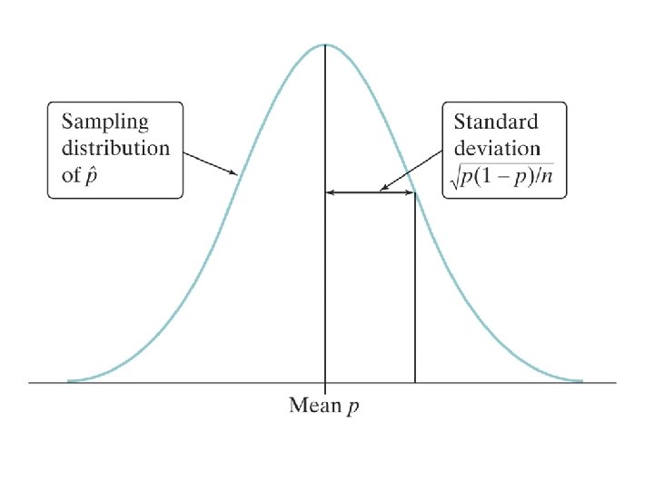
Confidence Intervals: Conditions 1) Random: The data should come from a well-designed random sample or randomized experiment. 2) Normal: The sampling distribution of the statistic is approximately Normal. For proportions: We can use the Normal approximation to the sampling distribution as long as np ≥ 10 and n(1 – p) ≥ 10. 3) Independent: Individual observations are independent. When sampling without replacement, the sample size n should be no more than 10% of the population size N (the 10% condition).

REVIEW: Finding a Critical Value Use Table A to find the critical value z* for an 80% confidence interval. Assume that the Normal condition is met. Since we want to capture the central 80% of the standard Normal distribution, we leave out 20%, or 10% in each tail. Search Table A to find the point z* with area 0. 1 to its left. The closest entry is z = – 1. 28. z . 07 . 08 . 09 – 1. 3 . 0853 . 0838 . 0823 – 1. 2 . 1020 . 1003 . 0985 – 1. 1 . 1210 . 1190 . 1170 So, the critical value z* for an 80% confidence interval is z* = 1. 28.

Common Confidence Intervals & zscores Confidence Level Z-Score 99% 95% 1. 96 90% We usually choose a confidence level of 90% or higher because we want to be quite sure of our conclusions. The most common confidence level is 95%.

Interpreting Confidence Levels The confidence level tells us how likely it is that the method we are using will produce an interval that captures the population parameter if we use it many times. For Example: “In 95% of all possible samples of the same size, the resulting confidence interval would capture the true (insert details in context). ” The confidence level does NOT tell us the chance that a particular confidence interval captures the population parameter. NO: There is a 95% chance that the mean is between….

Interpreting Confidence Intervals Interpret: “We are 95% confident that the interval from ______ to _______ captures the actual value of the (insert population parameter details…)” NOT There is a 95% percent chance…. For example: “We are 95% confident that the interval from 3. 03 inches to 3. 35 inches capture the actual mean amount of rain in the month of April in Miami. ”

Interpret the Following… According to www. gallup. com, on August 13, 2015, the 95% confidence interval for the true proportion of Americans who approved of the job Barack Obama was doing as president was 0. 44 +/- 0. 03. Interpret the confidence interval and level.

Interpret the Following… Interval: We are 95% confident that the interval from 0. 41 to 0. 47 captures the true proportion of Americans who approve of the job Barack Obama was doing as president at the time of the poll. Level: In 95% of all possible samples of the same size, the resulting confidence interval would capture the true proportion of Americans who approve of the job Barack Obama was doing as president.

Confidence Intervals: Properties The margin of error: (critical value) • (standard deviation) The margin of error gets smaller when: • The confidence level decreases • The sample size n increases

Confidence Intervals: Properties • The critical value (z-score) depends on the confidence level and the sampling distribution of the statistic. • Greater confidence requires a larger critical value • The standard deviation of the statistic depends on the sample size n

Section 8. 2 Estimating a Population Proportion

Section 8. 2 Estimating a Population Proportion After this section, you should be able to… ü CONSTRUCT and INTERPRET a confidence interval for a population proportion ü DETERMINE the sample size required to obtain a level C confidence interval for a population proportion with a specified margin of error ü DESCRIBE how the margin of error of a confidence interval changes with the sample size and the level of confidence C

Estimating p & Constructing a CI: Conditions 1) Random: The data should come from a well-designed random sample or randomized experiment. 3) Independent: Individual observations are independent. When sampling without replacement, the sample size n should be no more than 10% of the population size N (the 10% condition).

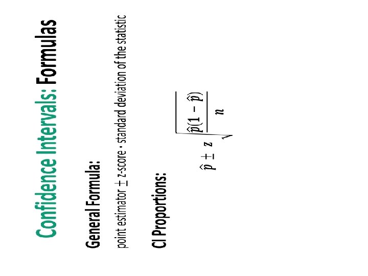
Formula: Confidence Interval for p

The Process: Confidence Intervals Parameter: p = true proportion…. Assess Conditions: Random: SRS or random assignment Sample Size: be sure to show both np ≥ 10 and n(1 – p) ≥ 10, the formula plugged and a sentence stating the values are greater than 10, therefore normal. Independent: 10% rule Name Interval: 1 -proportion z-Interval: Use your calculator. “We are ____% confident that the interval from ____ to ____ will capture the true proportion of (context)…” Conclude in Context: Answer the question being asked.

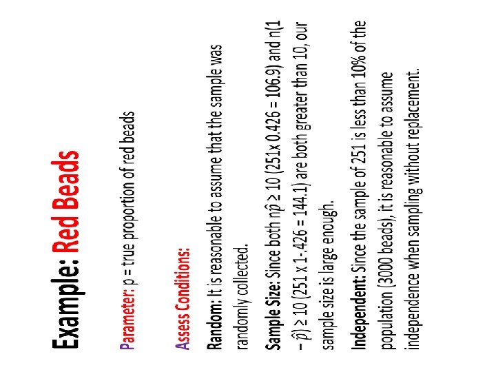
Example: Red Beads Calculate and interpret a 90% confidence interval for the proportion of red beads in the container of 3000 beads. Mrs. Daniel claims 50% of the beads are red. Use your interval to comment on this claim. The sample proportion you found was 0. 426 with a sample of 251 beads. z . 03 . 04 . 05 – 1. 7 . 0418 . 0409 . 0401 – 1. 6 . 0516 . 0505 . 0495 – 1. 5 . 0630 . 0618 . 0606 ü For a 90% confidence level, z* = 1. 645

Example: Red Beads Name Interval: 1 -proportion z-Interval: We are 90% confident that the interval from 0. 375 to 0. 477 will capture the true proportion of red beads. statistic ± (critical value) • (standard deviation of the statistic) 0. 426 +/- 1. 645 *

Example: Red Beads Name Interval: 1 -proportion z-Interval: We are 90% confident that the interval from 0. 375 to 0. 477 will capture the true proportion of red beads.

Example: Red Beads Conclude in Context: It is pretty doubtful that Mrs. Daniel’s claim in true that 50% of the beads are red because 0. 50 is not included within the interval.

2011 B #5 During a flu vaccine shortage in the United States, it was believed that 45 percent of vaccine-eligible people received flu vaccine. The results of a survey given to a random sample of 2, 350 vaccine-eligible people indicated that 978 of the 2, 350 people had received flu vaccine. (a) Construct a 99 percent confidence interval for the proportion of vaccine-eligible people who had received flu vaccine. Use your confidence interval to comment on the belief that 45 percent of the vaccine-eligible people had received flu vaccine.

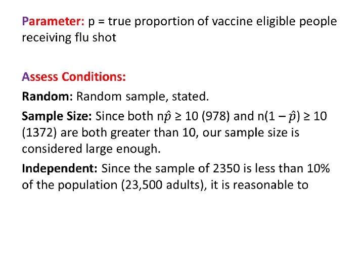
Name Interval: 1 -proportion z-Interval: We are 99% confident that the interval from 0. 38998 to 0. 44236 will capture the true proportion of vaccine eligible adults receiving the flu shot. Conclude in Context: Since 0. 45 (45%) is not contained within the interval, we have reasonable evidence that 45% of eligible adults did not get vaccinated.

Example: Customer Satisfaction Mc. Donald's wants to determine customer satisfaction with its new BBQ Chicken Burger. The VP of New Products has hired you to conduct a survey. At a minimum how many people do you need to survey, if the company is requiring a margin of error of 0. 03 at 95% confidence?

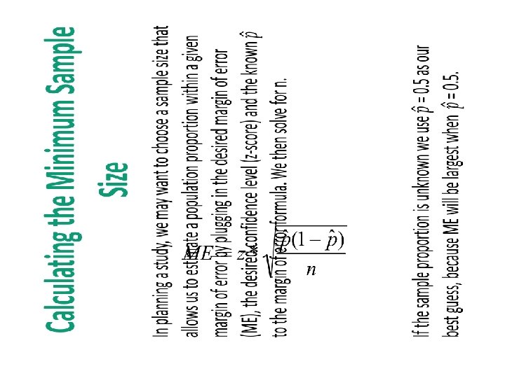
Example: Customer Satisfaction Mac. Donald's wants to determine customer satisfaction with its new BBQ Chicken Burger. The VP of New Products has hired you to conduct a survey. At a minimum how many people do you need to survey, if the company is requiring a margin of error of 0. 03 at 95% confidence? Multiply both sides by square root n and divide both sides by 0. 03. Square both sides. Substitute 0. 5 for the sample proportion to find the largest ME possible. We round up to 1068 respondents to ensure the margin of error is no more than 0. 03 at 95% confidence.

2011 B #5 b (b) Suppose a similar survey will be given to vaccine-eligible people in Canada by Canadian health officials. A 99 percent confidence interval for the proportion of people who will have received flu vaccine is to be constructed. What is the smallest sample size that can be used to guarantee that the margin of error will be less than or equal to 0. 02 ?

Solution The sample-size calculation uses 0. 5 as the value of the proportion in order to provide the minimum required sample size to guarantee that the resulting interval will have a margin of error no larger than 0. 02. A sample of at least 4, 148 vaccine-eligible people should be taken in Canada.

Section 9. 1 Significance Tests: The Basics

Section 9. 1 Significance Tests: The Basics After this section, you should be able to… ü STATE correct hypotheses for a significance test about a population proportion or mean. ü INTERPRET P-values in context.

Statistical Inference Significance Tests- Confidence Interval - • ASSESS the evidence provided by data about some claim concerning a population • Reject or fail to reject (Yes vs. No) • ESTIMATE a population parameter. • Give range of possible values

Significance Test A significance test is a formal procedure for comparing observed data with a claim (also called a hypothesis) whose truth we want to assess. The claim is a statement about a parameter, like the population proportion p or the population mean µ. We express the results of a significance test in terms of a probability (p-value) that measures how well the data and the claim agree.

The Reasoning of Significance Tests Statistical tests deal with claims about a population. Tests ask if sample data give good evidence against a claim. A test might say, “If we took many random samples and the claim were true, what is the probability we will get a result like this. ” For example: Suppose a basketball player claimed to be an 80% free-throw shooter. To test this claim, we have him attempt 50 free-throws. He makes 32 of them. His sample proportion of made shots is 32/50 = 0. 64. What can we conclude about the claim based on this sample data? What is the probability the player is telling the truth? !? !

The Reasoning of Significance Tests We can use software to simulate 400 sets of 50 shots assuming that the player is really an 80% shooter.

The Reasoning of Significance Tests You can say how strong the evidence against the player’s claim is by giving the probability that he would make as few as 32 out of 50 free throws if he really makes 80% in the long run. The observed statistic is so unlikely if the actual parameter value is p = 0. 80 that it gives convincing evidence that the player’s claim is not true.

The Reasoning of Significance Tests Based on the evidence, we might conclude the player’s claim is incorrect. In reality, there are two possible explanations for the fact that he made only 64% of his free throws. 1) The player’s claim is correct (p = 0. 8), and by horrible luck, a very unlikely outcome occurred. 2) The population proportion is actually less than 0. 8, so the sample result is not an unlikely outcome. Basic Idea An outcome that would rarely happen if a claim were true is good evidence that the claim is not true.

Stating Hypotheses The claim tested by a statistical test is called the null hypothesis (H 0). The test is designed to assess the strength of the evidence against the null hypothesis. Often the null hypothesis is a statement of “no difference” or that the claim is true. The claim about the population that we are trying to find evidence for is the alternative hypothesis (Ha). In the free-throw shooter example, our hypotheses are H 0 : p = 0. 80 Ha : p < 0. 80 Parameter: p = the long-run proportion of made free throws.

Stating Hypotheses In any significance test, the null hypothesis has the form H 0 : parameter = value The alternative hypothesis has one of the forms Ha : parameter < value Ha : parameter > value Ha : parameter ≠ value To determine the correct form of Ha, read the problem carefully.

Stating Hypotheses

State the Hypothesis & Parameter: A high school junior running for student body president, Sally, claims that 70% of the student body favors her in the school election. Her opponent believes this percentage to be lower, write the appropriate null and alternative hypotheses.

State the Hypothesis & Parameter: p= true proportion of students that favor Sally for president.

Interpreting P-Values • The null hypothesis H 0 states the claim that we are seeking evidence against. • The probability that measures the strength of the evidence against a null hypothesis is called a P-value. • The probability, computed assuming H 0 is true, that the statistic would take a value as extreme as or more extreme than the one actually observed is called the Pvalue of the test. • The smaller the P-value, the stronger the evidence against H 0 provided by the data.

H 0: µ = 0 English Math Small P-value Evidence against Unlikely to occur if H 0 is true We reject H 0 Large P-value Not convincing evidence Could occur if We fail to H 0 is true reject H 0

Example: Studying Job Satisfaction Does the job satisfaction of assembly-line workers differ when their work is machine-paced rather than self-paced? One study chose 18 subjects at random from a company with over 200 workers who assembled electronic devices. Half of the workers were assigned at random to each of two groups. Both groups did similar assembly work, but one group was allowed to pace themselves while the other group used an assembly line that moved at a fixed pace. After two weeks, all the workers took a test of job satisfaction. Then they switched work setups and took the test again after two more weeks. The response variable is the difference in satisfaction scores, self-paced minus machine-paced. a) Describe the parameter of interest in this setting. b) State appropriate hypotheses for performing a significance test.

Example: Studying Job Satisfaction a) Describe the parameter of interest in this setting. The parameter of interest is the mean µ of the differences (self-paced minus machine-paced) in job satisfaction scores in the population of all assembly-line workers at this company. (FYI- Matched pairs!!!) b) State appropriate hypotheses for performing a significance test. Because the initial question asked whether job satisfaction differs, the alternative hypothesis is two-sided; that is, either µ < 0 or µ > 0. For simplicity, we write this as µ ≠ 0. That is, H 0 : µ = 0 Ha : µ ≠ 0

Example: Studying Job Satisfaction For the job satisfaction study, the hypotheses are H 0: µ = 0 H a: µ ≠ 0 c) Explain what it means for the null hypothesis to be true in this setting. d) Interpret the given P-value in context.

Example: Studying Job Satisfaction For the job satisfaction study, the hypotheses are H 0 : µ = 0 Ha : µ ≠ 0 c) Explain what it means for the null hypothesis to be true in this setting. In this setting, the null hypothesis is that there is no mean difference in employee satisfaction scores (self-paced machine-paced) for the entire population of assemblyline workers at the company. If null hypothesis is true, then the workers don’t favor one work environment over the other, on average.

Example: Studying Job Satisfaction d) Interpret the P-value in context. The P-value is the probability of observing a sample result as extreme as (or more extreme) by pure chance given that the null hypothesis is actually true. Since the test is two-sided, we have a 23% chance of observing a value that is 17 points or more from the mean, in either direction. An outcome that would occur so often just by chance (almost 1 in every 4 random samples of 18 workers) when the null is true is not convincing evidence against null. We fail to reject H 0: µ = 0.

Conclusion: Statistical Significance We will make one of two decisions based on the strength of the evidence against the null hypothesis (and in favor of the alternative hypothesis) -- reject H 0 or fail to reject H 0. ü If our sample result is too unlikely to have happened by chance assuming H 0 is true, then we’ll reject H 0. ü Otherwise, we will fail to reject H 0. A fail-to-reject H 0 decision in a significance test doesn’t mean that H 0 is true. For that reason, you should never “accept H 0” or use language implying that you believe H 0 is true.

Statistically Significant • There is no perfect rule for how small a P-value we should require in order to reject H 0 — it’s a matter of judgment and depends on the specific circumstances. • We can compare the P-value with a fixed value (typically α = 0. 05), called the significance level (alpha α). • When our p-value is greater than the chosen α, there is no statistically significance. We “fail to reject” the null. • When our P-value is less than the chosen α, we say that the result is statistically significant. – In that case, we reject the null hypothesis H 0 and conclude that there is convincing evidence in favor of the alternative hypothesis Ha.

General conclusion in a significance test : P-value small → reject H 0 → conclude Ha P-value large → fail to reject H 0 → cannot conclude Ha Conclusion with fixed level of significance : P-value < α → reject H 0 → conclude Ha P-value ≥ α → fail to reject H 0 → cannot conclude Ha

Example: Better Batteries A company has developed a new deluxe AAA battery that is supposed to last longer than its regular AAA battery. However, these new batteries are more expensive to produce, so the company would like to be convinced that they really do last longer. Based on years of experience, the company knows that its regular AAA batteries last for 30 hours of continuous use, on average. The company selects an SRS of 15 new batteries and uses them continuously until they are completely drained. A significance test is performed using the hypotheses H 0 : µ = 30 hours Ha : µ > 30 hours where µ is the true mean lifetime of the new deluxe AAA batteries. The resulting P-value is 0. 0276. a) What conclusion can you make for the significance level α = 0. 05? b) What conclusion can you make for the significance level α = 0. 01?

Example: Better Batteries a) What conclusion can you make for the significance level α = 0. 05? Since the P-value, 0. 0276, is less than α = 0. 05, the sample result is statistically significant at the 5% level. We have sufficient evidence to reject the null hypothesis and have sufficient evidence to conclude that the company’s deluxe AAA batteries last longer than 30 hours, on average. b) What conclusion can you make at significance level α = 0. 01? Since the P-value, 0. 0276, is greater than α = 0. 01, the sample result is not statistically significant at the 1% level. We fail to reject the null hypothesis; therefore, we cannot conclude that the deluxe AAA batteries last longer than 30 hours, on average.

Section 9. 1 Significance Tests: The Basics ü A significance test assesses the evidence provided by data against a null hypothesis H 0 in favor of an alternative hypothesis Ha. ü The hypotheses are stated in terms of population parameters. Often, H 0 is a statement of no change or no difference. Ha says that a parameter differs from its null hypothesis value in a specific direction (one-sided alternative) or in either direction (two-sided alternative). ü The reasoning of a significance test is as follows. Suppose that the null hypothesis is true. If we repeated our data production many times, would we often get data as inconsistent with H 0 as the data we actually have? If the data are unlikely when H 0 is true, they provide evidence against H 0. ü The P-value of a test is the probability, computed supposing H 0 to be true, that the statistic will take a value at least as extreme as that actually observed in the direction specified by Ha.

Section 9. 1 Significance Tests: The Basics Summary ü Small P-values indicate strong evidence against H 0. To calculate a Pvalue, we must know the sampling distribution of the test statistic when H 0 is true. There is no universal rule for how small a P-value in a significance test provides convincing evidence against the null hypothesis. ü If the P-value is smaller than a specified value α (called the significance level), the data are statistically significant at level α. In that case, we can reject H 0. If the P-value is greater than or equal to α, we fail to reject H 0.

Section 9. 2 Tests About a Population Proportion

Section 9. 2 Tests About a Population Proportion After this section, you should be able to… ü CHECK conditions for carrying out a test about a population proportion. ü CONDUCT a significance test about a population proportion. ü CONSTRUCT a confidence interval to draw a conclusion about for a two-sided test about a population proportion.

Carrying Out a Significance Test Recall our basketball player who claimed to be an 80% free-throw shooter. In an SRS of 50 freethrows, he made 32. His sample proportion of made shots, 32/50 = 0. 64, is much lower than what he claimed. Does it provide convincing evidence against his claim? We use z-scores and p-values to evaluate.

Theory: One-Sample z Test for a Proportion The z statistic has approximately the standard Normal distribution when H 0 is true.

Theory: Test Statistic and P-value A significance test uses sample data to measure the strength of evidence against H 0. • The test compares a statistic calculated from sample data with the value of the parameter stated by the null hypothesis. • Values of the statistic far from the null parameter value in the direction specified by the alternative hypothesis give evidence against H 0. • A test statistic measures how far a sample statistic diverges from what we would expect if the null hypothesis H 0 were true.

Carrying Out a Significance Test P Parameters H Hypothesis A Assess Conditions N T Name the Test O Obtain P-value M Make a decision S State conclusion Test Statistic (Calculate)

Carrying Out a Significance Test Parameters & Hypothesis Parameter: p = the actual proportion of free throws the shooter makes in the long run. Hypothesis: H 0: p = 0. 80 Ha: p < 0. 80

Carrying Out a Significance Test Assess Conditions: Random, Normal & Independent. ü Random We can view this set of 50 shots as a simple random sample from the population of all possible shots that the player takes. ü Normal Assuming H 0 is true, p = 0. 80. then np = (50)(0. 80) = 40 and n (1 - p) = (50)(0. 20) = 10 are both at least 10, so the normal condition is met. ü Independent In our simulation, the outcome of each shot does is determined by a random number generator, so individual observations are independent.

Carrying Out a Significance Test Name the Test, Test Statistic (Calculate) & Obtain P-value Name Test: One-proportion z-test Z- score: -2. 83 P- value: 0. 0023

Carrying Out a Significance Test Make a Decision & State the Conclusion Make a Decision: P-value is 0. 0023. Since the p-value is so small we reject the null hypothesis. State the Conclusion: We have convincing evidence that the basketball player does not make 80% of his free throws.

Example: One Potato, Two Potato A potato-chip producer has just received a truckload of potatoes from its main supplier. If the producer determines that more than 8% of the potatoes in the shipment have blemishes, the truck will be sent away to get another load from the supplier. A supervisor selects a random sample of 500 potatoes from the truck. An inspection reveals that 47 of the potatoes have blemishes. Carry out a significance test at the α= 0. 10 significance level. What should the producer conclude?

Example: One Potato, Two Potato State Parameter & State Hypothesis α = 0. 10 significance level Parameter: p = actual proportion of potatoes in this shipment with blemishes. Hypothesis: H 0: p = 0. 08 Ha: p > 0. 08

Example: One Potato, Two Potato Assess Check Conditions üRandom sample of 500 potatoes üNormal Assuming H 0: p = 0. 08 is true, the expected numbers of blemished and unblemished potatoes are np 0 = 500(0. 08) = 40 and n(1 - p 0) = 500(0. 92) = 460, respectively. Because both of these values are at least 10, we should be safe doing Normal calculations. üIndependent Because we are sampling without replacement, we need to check the 10% condition. It seems reasonable to assume that there at least 10(500) = 5000 potatoes in the shipment.

Example: One Potato, Two Potato Make a Decision and State Conclusion Make a Decision: Since our P-value, 0. 1251, is greater than the chosen significance level of α = 0. 10, so we fail to reject the null hypothesis. State Conclusion: There is not sufficient evidence to conclude that the shipment contains more than 8% blemished potatoes. The producer will use this truckload of potatoes to make potato chips.

Smoking in High School According to the Centers for Disease Control and Prevention (CDC) Web site, 50% of high school students have never smoked a cigarette. Taeyeon wonders whether this national result holds true in his large, urban high school. For his AP Statistics class project, Taeyeon surveys an SRS of 150 students from his school. He gets responses from all 150 students, and 90 say that they have never smoked a cigarette. What should Taeyeon conclude? Give appropriate evidence to support your answer.

State Parameter & State Hypothesis Perform at test at the α = 0. 05 significance level Parameter: p = actual proportion of students in Taeyeon’s school who would say they have never smoked cigarettes Hypothesis: H 0: p = 0. 50 Ha: p ≠ 0. 50

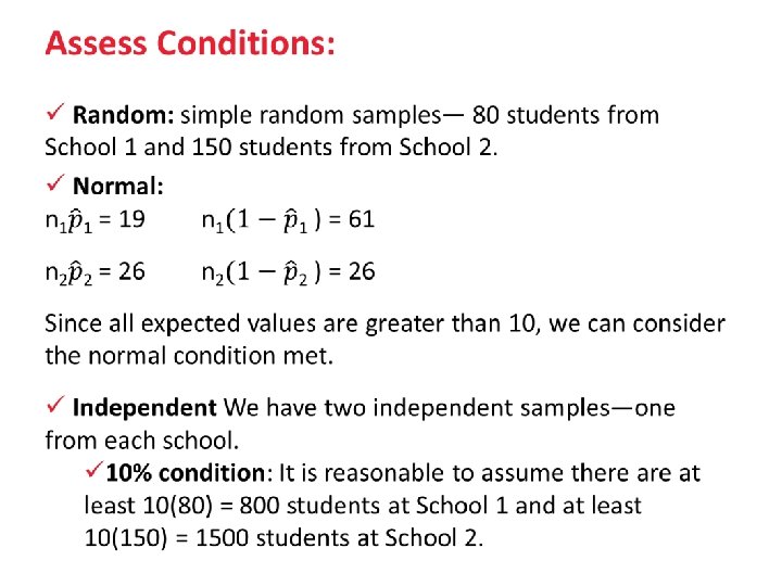
Assess Conditions üRandom Taeyeon surveyed an SRS of 150 students from his school. üNormal Assuming H 0: p = 0. 50 is true, the expected numbers of smokers and nonsmokers in the sample are np 0 = 150(0. 50) = 75 and n(1 - p 0) = 150(0. 50) = 75. Because both of these values are at least 10, we should be safe doing Normal calculations. üIndependent We are sampling without replacement, we need to check the 10% condition. It seems reasonable to assume that there at least 10(150) = 1500 students a large high school.

Carrying Out a Significance Test Name the Test, Test Statistic (Calculate) & Obtain P-value Name: One Proportion Z- Test P 0: 0. 50 x: 90 n: 150 Test Statistic: z = 2. 449 Obtain p-value: p = 0. 0143

Make a Decision & State Conclusion Make Decision: Since our P-value, 0. 0143, is less than the chosen significance level of α = 0. 05. we have sufficient evidence to reject H 0. State Conclusion: We have convincing evidence to conclude that the proportion of students at Taeyeon’s school who say they have never smoked differs from the national result of 0. 50.

Confidence Intervals Give More Information The result of a significance test is basically a decision to reject H 0 or fail to reject H 0. When we reject H 0, we’re left wondering what the actual proportion p might be. A confidence interval might shed some light on this issue. High School Smoking; our 95% confidence interval is: We are 95% confident that the interval from 0. 522 to 0. 678 captures the true proportion of students at Taeyeon’s high school who would say that they have never smoked a cigarette.

Confidence Intervals and Two. Sided Tests

Confidence Intervals and Two. Sided Tests

One Proportion Z-Test by Hand

Basketball- Carrying Out a Significance Test Step 3 a: Calculate Mean & Standard Deviation If the null hypothesis H 0 : p = 0. 80 is true, then the player’s sample proportion of made free throws in an SRS of 50 shots would vary according to an approximately Normal sampling distribution with mean

Basketball- Carrying Out a Significance Test Step 3 b: Calculate Test Statistic Then, Using Table A, we find that the P-value is P(z ≤ – 2. 83) = 0. 0023.

Example: One Potato, Two Potato Step 3: Calculations The sample proportion of blemished potatoes is P-value Using Table A the desired P-value is P(z ≥ 1. 15) = 1 – 0. 8749 = 0. 1251

High School Smoking The sample proportion is P-value To compute this Pvalue, we find the area in one tail and double it. Using Table A or normalcdf(2. 45, 100) yields P(z ≥ 2. 45) = 0. 0071 (the righttail area). So the desired P-value is 2(0. 0071) = 0. 0142.

10. 1 Comparing Two Proportions

Section 10. 1 Comparing Two Proportions After this section, you should be able to… ü DETERMINE whether the conditions for performing inference are met. ü CONSTRUCT and INTERPRET a confidence interval to compare two proportions. ü PERFORM a significance test to compare two proportions. ü INTERPRET the results of inference procedures in a randomized experiment.

Introduction • Helps us compare the proportions of individuals with a certain characteristic in two different populations. • We can compare proportions in both surveys and experiments. • Sample sizes nor population sizes need to be the same.

Theory: The Sampling Distribution of a Difference Between Two Proportions The sampling distribution of a sample proportion has the following properties: Shape Approximately Normal if np ≥ 10 and n(1 - p) ≥ 10

Theory: The Sampling Distribution of a Difference Between Two Proportions To explore the sampling distribution of the difference between two proportions, let’s start with two populations having a known proportion of successes. ü At School 1, 70% of students did their homework last night ü At School 2, 50% of students did their homework last night. Suppose the counselor at School 1 takes an SRS of 100 students and records the sample proportion that did their homework. School 2’s counselor takes an SRS of 200 students and records the sample proportion that did their homework.

Theory: The Sampling Distribution of a Difference Between Two Proportions Using Fathom software, we generated an SRS of 100 students from School 1 and a separate SRS of 200 students from School 2. The difference in sample proportions was then calculated and plotted. We repeated this process 1000 times. The results are below:

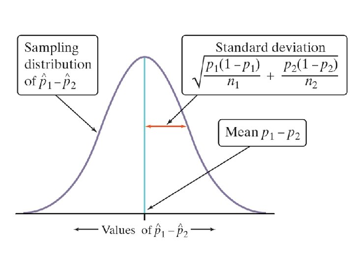
Formula: Confidence Intervals for p 1 – p 2

Conditions: Two Proportion ZInterval CI 1) Random: Both sets of data should come from a well-designed random samples or randomized experiments. 3) Independent: Both sets of data must be independent. When sampling without replacement, the sample size n should be no more than 10% of the population size N (the 10% condition). Must check the condition for each separate sample.

Let’s Practice: Teens and Adults on Social Networks As part of the Pew Internet and American Life Project, researchers conducted two surveys in late 2009. The first survey asked a random sample of 800 U. S. teens about their use of social media and the Internet. A second survey posed similar questions to a random sample of 2253 U. S. adults. In these two studies, 73% of teens and 47% of adults said that they use social-networking sites. Use these results to construct and interpret a 95% confidence interval for the difference between the proportion of all U. S. teens and adults who use social-networking sites.

Teens and Adults on Social Networks Parameters: p 1 = proportion of teens using social media p 2 = proportion of adults using social media Assess Conditions: ü Random The data come from two separate random samples ü Normal: the Normal condition is met since all counts are all at least 10: ü Independent We clearly have two independent samples—one of teens and one of adults. Individual responses in the two samples also have to be independent. ü 10% condition: We can reasonably assume that there at least 10(800) = 8000 U. S. teens and at least 10(2253) = 22, 530 U. S. adults.

Teens and Adults on Social Networks Name the Interval: 2 -proprtion z-Confidence Interval: We are 95% confident that the interval from 0. 223 to 0. 297 captures the true difference in the proportion of all U. S. teens and adults who use social-networking sites. Conclude: This interval suggests that more teens than adults in the United States engage in social networking by between 22. 3 and 29. 7 percentage points.

Significance Tests for p 1 – p 2 • An observed difference between two sample proportions can reflect an actual difference in the parameters, or it may just be due to chance variation in random sampling or random assignment. • Significance tests help us decide which explanation makes more sense. • The null hypothesis has the general form: H 0: p 1 = p 2 • The alternative hypothesis says what kind of difference we expect. Ha: p 1 > p 2 or Ha: p 1 < p 2 or Ha: p 1 ≠ p 2

Significance Tests for p 1 – p 2

Significance Tests for p 1 – p 2

Why Do We Pool? “We have merged the data from the two samples to obtain what is called the "pooled" estimate of the standard deviation. We have done this not because it is more convenient (it isn't -- there's more calculation involved) nor because it reduces the measurement of variability (it doesn't always -- often the pooled estimate is larger*) but because it gives us the best estimate of the variability of the difference under our null hypothesis that the two sample proportions came from populations with the same proportion. ” For more details see: http: //apcentral. collegeboard. com/apc/members/courses/te achers_corner/49013. html

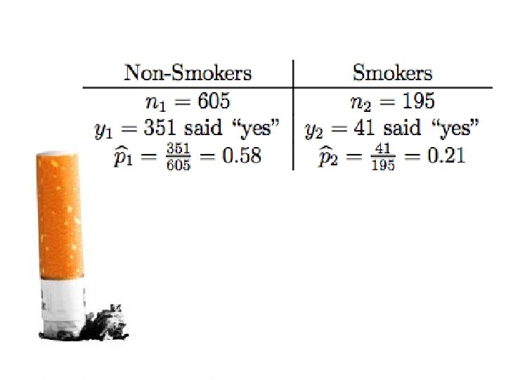
School Breakfast Researchers designed a survey to compare the proportions of children who come to school without eating breakfast in two low-income elementary schools. An SRS of 80 students from School 1 found that 19 had not eaten breakfast. At School 2, an SRS of 150 students included 26 who had not had breakfast. More than 1500 students attend each school. Do these data give convincing evidence of a difference in the population proportions? Carry out a significance test at the α = 0. 05 level to support your answer.

Hungry Children Parameters & Hypotheses: H 0 : p 1 = p 2 Ha : p 1 ≠ p 2 p 1 = the true proportion of students at School 1 who did not eat breakfast p 2 = the true proportion of students at School 2 who did not eat breakfast.

Name Test: Two-proportion z test Test Statistic: z = 1. 17 Obtain p-value: p = 0. 2426 Make a Decision: Since our P-value, 0. 2420, is greater than the chosen significance level of α = 0. 05, we fail to reject H 0. Conclude: There is not sufficient evidence to conclude that the proportions of students at the two schools who didn’t eat breakfast are different.

Colon Cancer: FRQ 2015 # 4

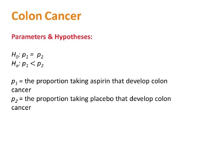
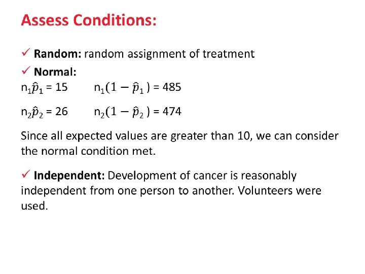
Name Test: Two-proportion z test Test Statistic: z = -1. 75 Obtain p-value: p = 0. 0396 Make a Decision: Since our P-value, 0. 0396, is less than the chosen significance level of α = 0. 05, we reject the null. Conclude: There is sufficient evidence to conclude that taking low does aspirin each day reduces the chance of developing colon cancer among all people similar to volunteers.

Scoring: 1. Parameters & Hypothesis – Direction must be correct – Must be in present tense (NO: developed cancer, took aspirin, had cancer, etc. ) 2. Name of Test, Conditions (random & normal) – Random Assignment (NO: stated or SRS) – Normal must have formula, values and sentence 3. Test Statistic & P-value 4. Decision, p-value linked to alpha & Context – NO proves, proven or for ALL people, etc.

Standard Error

Confidence Intervals for p 1 – p 2 If the Normal condition is met, we find the critical value z* for the given confidence level from the standard Normal curve. Our confidence interval for p 1 – p 2 is: