Section 6 Recursively defined functions Semantics of Loops

Section 6 Recursively defined functions

Semantics of Loops B: Boolean expression C: Command. . . C : : =. . . | while B do C |. . . C[[while B do C]] = s: B[[B]]s C[[while B do C]](C[[C]]s)[]s Problem: meaning of a syntax phrase may be defined only in terms of its proper sub parts.

C[[while B do C]] = w where w: Store w = s: B[[B]]s w(C[[C]]s) [] s Recursion in syntax exchanged for recursion in function notation!

Recursive Function Definitions • Function Definition – q = n: n equals zero one [] q(n plus one) • Possible Function Graphs: {(zero, one)} = {(zero, one), (one, ), (two, ), . . . } {(zero, one), (one, six), (two, six), . . . } {(zero, one), (one, k), (two, k), . . . } • Several functions satisfy specification; which one shall we choose?

Least Fixed Point Semantics Establishes meaning of recursive specifications: • Guarantees that every specification has a function satisfying it. • Provides means for choosing the ``best'' function out of the set of possibilities. • Ensures that the selected function corresponds to the conventional operational treatment of recursion. Argument is mapped to defined answer iff simplification of the specification yields a result in a finite number of recursive invocations.

The Factorial Function fac(n) = n equals zero one [] n times (fac(n minus one)) Only one function satisfies specification: graph(factorial) = {(zero, one), (one, one), (two, two), (three, six), . . . , (i, i!), . . . }

fac(three) three equals zero one [] three times fac(three minus one) = three times fac(two) three times (two equals zero one [] two times fac(two minus one)) = three times (two times fac(one)) three times (two times (one equals zero one [] one times fac(one minus one))) = three times (two times one (times fac(zero))) three times(two times(one times(zero equals zero one [] zero times fac(zero minus one)))) = three times (two times one (times one)) = six

Partial Functions • Answer is produced in a finite number of unfolding steps. • Idea: place limit on number of unfoldings and investigate resulting graphs – – zero: {} one: {(zero, one)} two: {(zero, one), (one, one)} i + 1: {(zero, one), (one, one), . . . (i, i!)}

• Graph at stage i defines function fac i. – Consistency with each other: • graph(fac i) graph(fac i+1) – Consistency with ultimate solution: • graph(fac i) graph(factorial) – Consequently • i=0 … infinity: graph(fac i ) graph(factorial)

Partial Functions Any result is computed in a finite number of unfoldings. • (a, b) graph(factorial) (a; b) graph(faci) (for some i) • Consequently graph(factorial) i=0 … infinity: graph(fac i ) Factorial function can be totally understood in terms of the finite subfunctions fac i !

Partial Functions • Representations of sub functions – fac 0 = n: – fac i+1 = n: n equals zero one [] n times fac i (n minus one) • Each definition is non recursive – Recursive specification can be understood in terms of a family of non recursive ones.

• Common format can be extracted – ``Functional'' F – F: (Nat ) – F = f: n: n equals zero one [] n times f(n minus one) • Each subfunction is an instance of the functional!

Functional and Fixed Point • Partial functions fac i+1 = F(fac i ) = Fi ( ) : = ( n: ) • Function graph(factorial) = i=0 … infinity: graph(Fi ( )) • Fixed point property graph(F(factorial)) = graph(factorial) F(factorial) = factorial • The function factorial is a fixed point of the functional F!

q Function • Q = q: n: n equals zero one [] q(n plus one) • Q 0( ) = ( n: ) • graph(Q 0( )) = {} • Q 1( ) = n: n equals zero one [] ( n: )(n plus one) = n: n equals zero one [] graph(Q 1( )) = {(zero, one)} • Q 2( )= Q(Q 1( ))) = n: n equals zero one []((n plus one) equals zero one [] ) • graph(Q 2( )) = {(zero, one)}

q Function • Convergence has occured – graph(Qi ( )) = {(zero, one)}, i >= 1 • Resulting graph – i=0 … inf: graph(Qi ( )) = {(zero; one)} • Fix point property – Q(qlimit) = qlimit • Still many solutions possible – graph(qk) = {(zero, one), (one, k), . . . , (i, k), . . . } • Least fixed point property – graph(qlimit) graph(qk) • The function qlimit is the least fixed point • of the functional Q!

Recursive Specifications • The meaning of a recursive specification f = F (f) is taken to be fix(F ), the least fixed point of the functional denoted by F. – graph(fix F) = i=0 … inf: graph(Fi ( )) • The domain D of F must be a pointed cpo – partial ordering on D, – every chain in D has a least upper bound in D – D has a least element.

• F must be continuous – Preserves limits of chains. • Semantic domains are cpos and their operations are continuous. – Pointed cpos are created from primitive domains and union domains by lifting.

Partial Ordering • The theory is formalised if the subset relation used within the fct graphs is generalised to a partial ordering. Then elements of semantic domains can be directly involved in set theoretical reasoning • A relation <= : D x D B is a PO upon D iff it is – reflexive – antisymetric – transitive • This allows us to treat the members of the domain D as if they are sets. • The partial ordering relation is read is “ is less defined than” • The symbol denotes the element in a PO domain that corresponds to the empty set.

Definitions: • Join/ least upper bound(lub): produces the smallest element that is larger than both of its arguments • Meet/greatest lower bound(glb): produces the largest (ie best defined) element that is smaller than both of its arguments. • Chain: A subset of a PO set is a chain iff the subset Is not empty and all elements of the subset are in a PO relation. • Complete Partial Ordering: a PO set D is a CPO iff every chain in D has a lub in D. • Pointed CPO: A partially ordered set D, is pointed cpo iff it is a complete partial ordering and it has a least element. • Monotonic: a <= b => f(a) <= f(b) • Continuous functions: Preserve limits on chains.

Join • For a partial ordering <= on Domain D, for all a, b D, a UNION b denotes the element of D if it exists such that: – a<= a UNION b and b <= a UNION b – for all d D, a <=d and b<= d imply a UNION b <=d – a UNION b id the join of a and b. The join operations produces the smallest element that is larger that both of its arguments. A PO might not have joins for all of its pairs. • Meet is defined in a similar way with x INTER y denoting the best defined element that is smaller than both x and y

• A functional F is a continuous function • The meaning of a recursive specification f = F(f) is taken to be fix F, the least fixpoint of the functional denoted by f.

Factorial Function • F = f. n. n equals zero one [] n times (f(n minus one)) • Simplification rule fix F = F(fix F)(three) = (F (fix F))(three) = ( f. n. n equals zero one[]n times(f(n minus one))(fix F))(three) = ( n. n equals zero one [] n times (fix F)(n minus one))(three) =

three equals zero one [] three times (fix F)(three minus one) = three times (fix F)(two) = three times (F (fix F))(two) =. . . = three times (two times (fix F)(two)) • Fixed point property justifies rec. unfolding!

Copyout function • Interactive text editor – copyout: Openfile File – copyout = (front, back). null front back [] copyout((tl front), ((hd front) cons back)) • Functional C, copyout = fix C. • With i unfoldings, list pairs of length i 1 can be appended. • Codomain is lifted because least fixed point semantics requires that the codomain of any recursively defined function be pointed. – ispointed(A B) = ispointed(B) – min(A B) = a. min(B)

Double Recursion g = n. n equals zero one [](g(n minus one) plus g(n minus one)) minus one graph(F 0( )) = {} graph(F 1( )) = {(zero, one)} graph(F 2( )) = {(zero, one), (one, one)} graph(F 3( )) = {(zero, one), (one, one), (two, one)} … graph(Fi+1( )) = {(zero, one), . . . , (i, one)} fix F = n. one Stepwise construction of graph yields insight!

While Loops • C[[while B do C]] = fix( f. s. B[[B]]s f(C[[C]]s) [] s) • Function: Store Example: C[[while A>0 do (A: =A 1; B: =B+1)]] = fix F where F = f. s: test s f(adjust s) [] s test = B[[A > 0]] adjust = C[[A: =A 1; B: =B+1]]

Partial function graphs: • Each pair in graph shows store prior to loop entry and after loop exit. • Each graph F i+1 ( ) contains those pairs whose input stores finish processing in at most i iterations.

While Loops Representation by finite subfunctions C[[while B do C]] = UNION { s. , s. B[[B]]s [] s, s. B[[B]]s (B[[B]](C[[C]]s) [] C[[C]]s)[]s, s. B[[B]]s (B[[B]](C[[C]]s)) [] C[[C]](C[[C]]s)) [] C[[C]]s) [] s, …} i. e. no guard evaluation, one guard evaluation, two guard evaluations etc.

= UNION { C[[diverge]], C[[if B then diverge else skip]], C [[ if B then (C; if B then diverge else skip) else skip]], C[[if B then (C; if B then diverge else skip) else skip]], …} Loop iteration can be understood by sequence of non iterating programs.

Reasoning about Least Fixed Points • Fixed Point Induction Principle: To prove P (fix F ), it suffices to prove 1. P ( ) 2. P (d) P (F (d)), for arbitrary d D for pointed cpo D, continuous functional F : D D, and inclusive predicate P : D B. • Inclusiveness of predicates If predicate holds for every element of chain, it also holds for its least upper bound.

• All universally quantified combinations of conjunctions/disjunctions that use only partial ordering over functional expressions are inclusive. • Mainly useful for showing equivalences of program constructs.

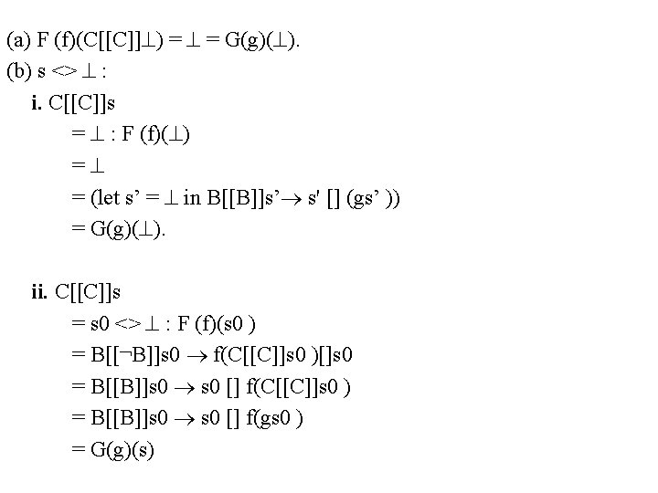
Reasoning about Least Fixed Points C[[repeat C until B]] = fix( f. s. let s’= C[[C]]s in B[[B]]s’!s’[](f s’)) C[[C; while ¬B do C]] = C[[repeat C until B]]? Proof: P(f, g) = s: f(C[[C]]s) = (gs) 1. P( , ) holds. 2. Prove P (F(f), G(g)) F = ( f. s. B[[¬ B]]s f(C[[C]]s) [] s) G = ( f. s. let s’ = C[[C]]s in B[[B]]s’ s’ [] (fs’ ))