Section 5 4 Sampling Distributions and the Central

Section 5. 4 Sampling Distributions and the Central Limit Theorem • Find sampling distributions and verify their properties • Interpret the Central Limit Theorem • Apply the Central Limit Theorem to find the probability of a sample mean Larson/Farber 1

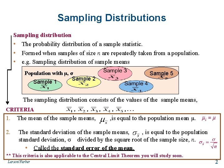
Sampling Distributions Sampling distribution • The probability distribution of a sample statistic. • Formed when samples of size n are repeatedly taken from a population. • e. g. Sampling distribution of sample means Population with μ, σ Sample 2 Sample 1 Sample 5 The sampling distribution consists of the values of the sample means, CRITERIA 1. The mean of the sample means, 2. The standard deviation of the sample means, , is equal to the population standard deviation, σ divided by the square root of the sample size, n. • Called the standard error of the mean. , is equal to the population mean μ. ** This criteria is also applicable to the Central Limit Theorem you will study soon. Larson/Farber 2

Sampling Distribution of Sample Means Example: The population values {1, 3, 5, 7} are written on slips of paper and put in a box. Two slips of paper are randomly selected, with replacement. All possible samples of size n = 2 and the mean of each sample. Sample 1, 1 1 Sample 5, 1 3 1, 3 2 5, 3 4 1, 5 3 5, 5 5 1, 7 4 5, 7 6 3, 1 2 7, 1 4 3, 3 3 4 7, 3 5 7, 5 6 5 7, 7 7 3, 5 3, 7 Sampling distribution of the means Probability distribution of Sample Mean 1 2 3 f 1 2 3 Probability 0. 0625 0. 1250 0. 1875 4 5 6 7 4 3 2 1 0. 2500 0. 1875 0. 1250 0. 0625 Satisfies Criteria of Sampling Distribution

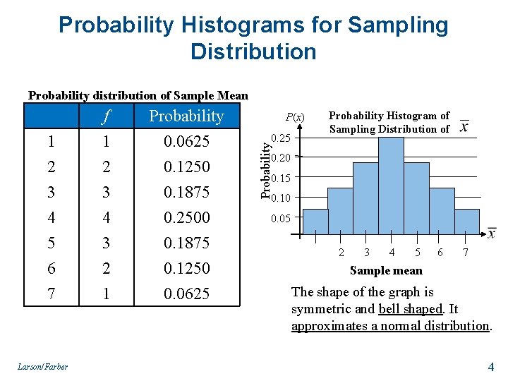
Probability Histograms for Sampling Distribution Probability distribution of Sample Mean Probability 0. 0625 0. 1250 0. 1875 4 5 6 7 4 3 2 1 0. 2500 0. 1875 0. 1250 0. 0625 Larson/Farber P(x) 0. 25 Probability Histogram of Sampling Distribution of Probability 1 2 3 f 1 2 3 0. 20 0. 15 0. 10 0. 05 2 3 4 5 6 7 Sample mean The shape of the graph is symmetric and bell shaped. It approximates a normal distribution. 4

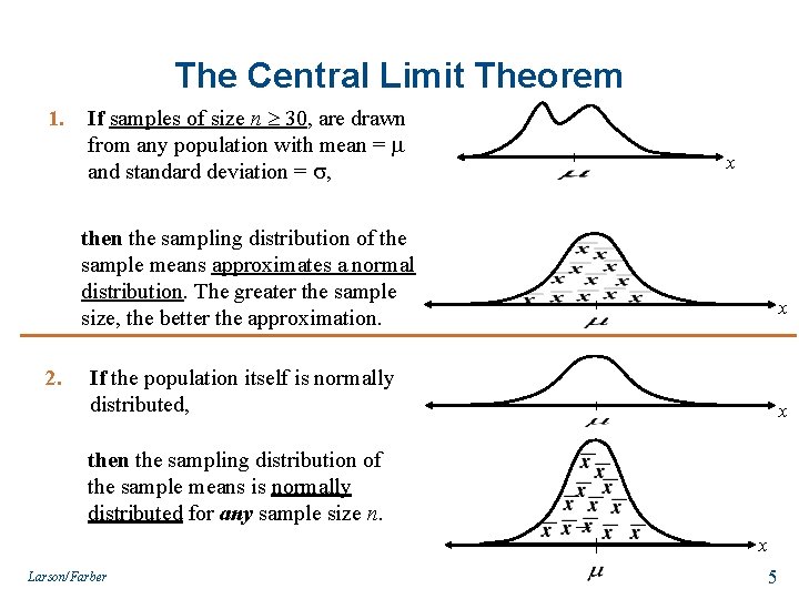
The Central Limit Theorem 1. If samples of size n 30, are drawn from any population with mean = and standard deviation = , x then the sampling distribution of the sample means approximates a normal distribution. The greater the sample size, the better the approximation. 2. x If the population itself is normally distributed, x then the sampling distribution of the sample means is normally distributed for any sample size n. x Larson/Farber 5

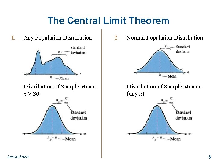
The Central Limit Theorem 1. Any Population Distribution of Sample Means, n ≥ 30 Larson/Farber 2. Normal Population Distribution of Sample Means, (any n) 6

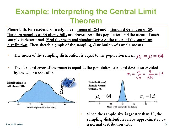
Example: Interpreting the Central Limit Theorem Phone bills for residents of a city have a mean of $64 and a standard deviation of $9. Random samples of 36 phone bills are drawn from this population and the mean of each sample is determined. Find the mean and standard error of the mean of the sampling distribution. Then sketch a graph of the sampling distribution of sample means. • The mean of the sampling distribution is equal to the population mean • The standard error of the mean is equal to the population standard deviation divided by the square root of n. • Larson/Farber Since the sample size is greater than 30, the sampling distribution can be approximated by a normal distribution with 7

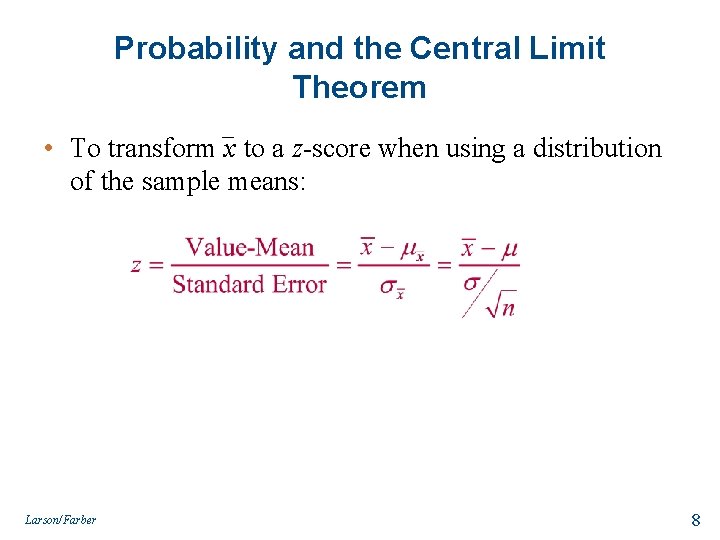
Probability and the Central Limit Theorem • To transform x to a z-score when using a distribution of the sample means: Larson/Farber 8

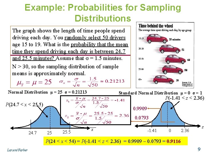
Example: Probabilities for Sampling Distributions The graph shows the length of time people spend driving each day. You randomly select 50 drivers age 15 to 19. What is the probability that the mean time they spend driving each day is between 24. 7 and 25. 5 minutes? Assume that σ = 1. 5 minutes. N > 30, so the sampling distribution of sample means is approximately normal. Normal Distribution μ = 25 σ = 0. 21213 Standard Normal Distribution μ = 0 σ = 1 P(-1. 41 < z < 2. 36) P(24. 7 < x < 25. 5) 0. 9909 0. 0793 24. 7 25 25. 5 x -1. 41 0 z 2. 36 P(24 < x < 54) = P(-1. 41 < z < 2. 36) = 0. 9909 – 0. 0793 = 0. 9116 Larson/Farber 9

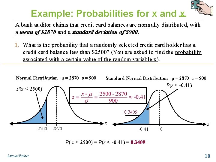
Example: Probabilities for x and x A bank auditor claims that credit card balances are normally distributed, with a mean of $2870 and a standard deviation of $900. 1. What is the probability that a randomly selected credit card holder has a credit card balance less than $2500? (You are asked to find the probability associated with a certain value of the random variable x). Normal Distribution μ = 2870 σ = 900 Standard Normal Distribution μ = 2870 σ = 900 P(z < -0. 41) P(x < 2500) 0. 3409 x 2500 2870 -0. 41 0 z P( x < 2500) = P(z < -0. 41) = 0. 3409 Larson/Farber 10

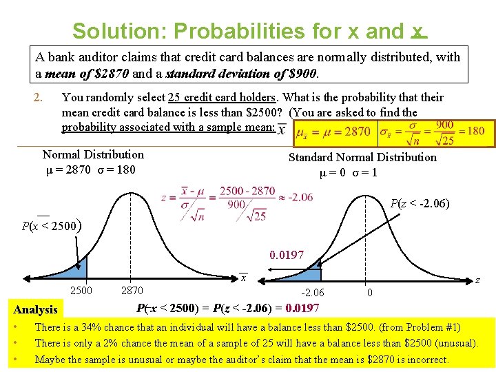
Solution: Probabilities for x and x A bank auditor claims that credit card balances are normally distributed, with a mean of $2870 and a standard deviation of $900. 2. You randomly select 25 credit card holders. What is the probability that their mean credit card balance is less than $2500? (You are asked to find the probability associated with a sample mean: Normal Distribution μ = 2870 σ = 180 Standard Normal Distribution μ=0 σ=1 P(z < -2. 06) P(x < 2500) 0. 0197 x 2500 Analysis • • • 2870 z -2. 06 0 P( x < 2500) = P(z < -2. 06) = 0. 0197 There is a 34% chance that an individual will have a balance less than $2500. (from Problem #1) There is only a 2% chance the mean of a sample of 25 will have a balance less than $2500 (unusual). Maybe the sample is unusual or maybe the auditor’s claim that the mean is $2870 is incorrect.