Section 4 6 The Derivative in Graphing and

Section 4. 6 The Derivative in Graphing and Applications: “Rectilinear Motion”

All graphics are attributed to: • Calculus, 10/E by Howard Anton, Irl Bivens, and Stephen Davis Copyright © 2009 by John Wiley & Sons, Inc. All rights reserved.

Introduction • Recall from section 2. 1 that a particle that can move in either direction along a coordinate line is said to be in rectilinear motion. • The line might be an x-axis, y-axis, or an axis inclined at some angle, therefore, we will call it a general “s-axis”.

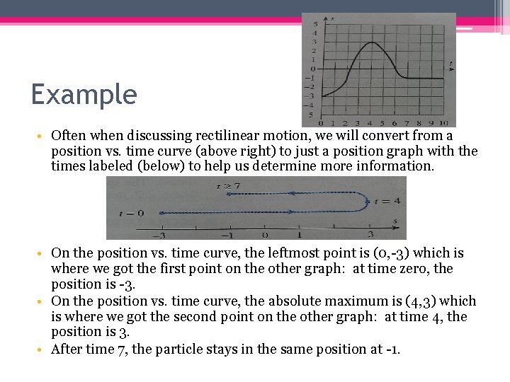
Example • Often when discussing rectilinear motion, we will convert from a position vs. time curve (above right) to just a position graph with the times labeled (below) to help us determine more information. • On the position vs. time curve, the leftmost point is (0, -3) which is where we got the first point on the other graph: at time zero, the position is -3. • On the position vs. time curve, the absolute maximum is (4, 3) which is where we got the second point on the other graph: at time 4, the position is 3. • After time 7, the particle stays in the same position at -1.

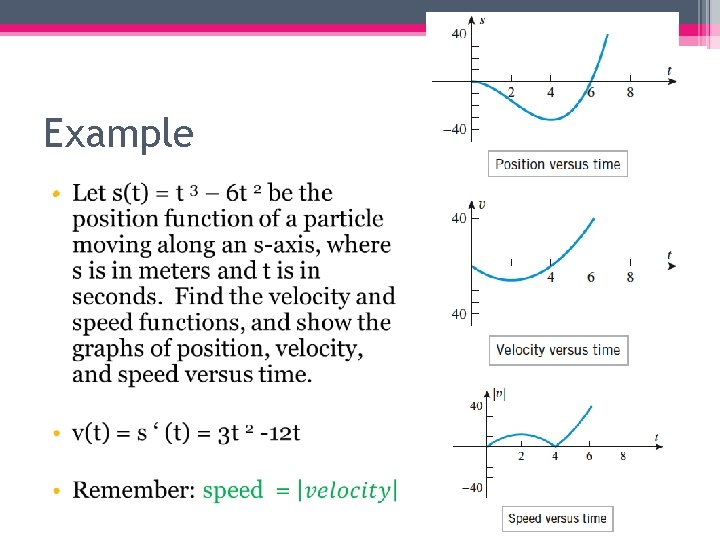
Velocity and Speed •

Example •

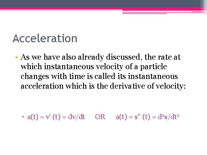
Acceleration • As we have also already discussed, the rate at which instantaneous velocity of a particle changes with time is called its instantaneous acceleration which is the derivative of velocity: ▫ a(t) = v’ (t) = dv/dt OR a(t) = s’’ (t) = d 2 s/dt 2

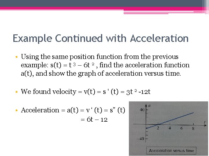
Example Continued with Acceleration • Using the same position function from the previous example: s(t) = t 3 – 6 t 2 , find the acceleration function a(t), and show the graph of acceleration versus time. • We found velocity = v(t) = s ‘ (t) = 3 t 2 -12 t • Acceleration = a(t) = v ‘ (t) = s” (t) = 6 t – 12

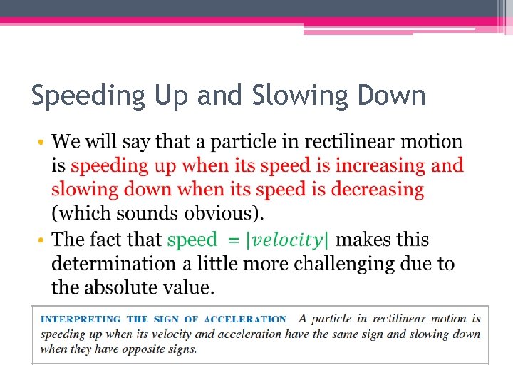
Speeding Up and Slowing Down •

Speeding Up and Slowing Down con’t • A particle with negative velocity is speeding up when its acceleration is negative (it is getting “more negative, faster”). • Likewise, a particle with negative velocity is slowing down when its acceleration is positive. • I find it easiest to make a number line and label where the velocity and acceleration are positive, negative, and zero (see next few slides).

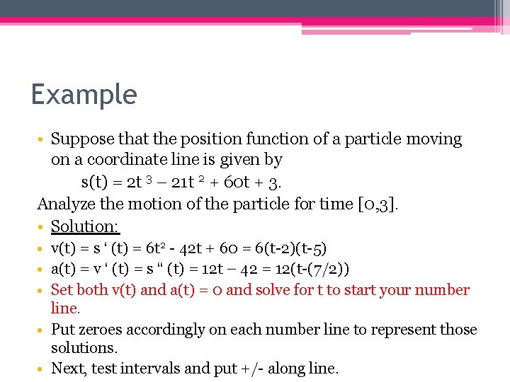
Example • Suppose that the position function of a particle moving on a coordinate line is given by s(t) = 2 t 3 – 21 t 2 + 60 t + 3. Analyze the motion of the particle for time [0, 3]. • Solution: • v(t) = s ‘ (t) = 6 t 2 - 42 t + 60 = 6(t-2)(t-5) • a(t) = v ‘ (t) = s “ (t) = 12 t – 42 = 12(t-(7/2)) • Set both v(t) and a(t) = 0 and solve for t to start your number line. • Put zeroes accordingly on each number line to represent those solutions. • Next, test intervals and put +/- along line.

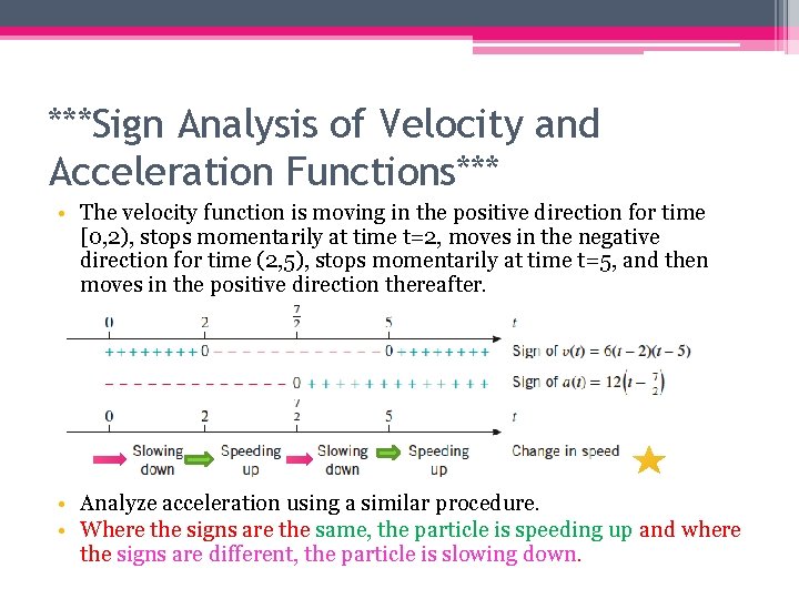
***Sign Analysis of Velocity and Acceleration Functions*** • The velocity function is moving in the positive direction for time [0, 2), stops momentarily at time t=2, moves in the negative direction for time (2, 5), stops momentarily at time t=5, and then moves in the positive direction thereafter. • Analyze acceleration using a similar procedure. • Where the signs are the same, the particle is speeding up and where the signs are different, the particle is slowing down.

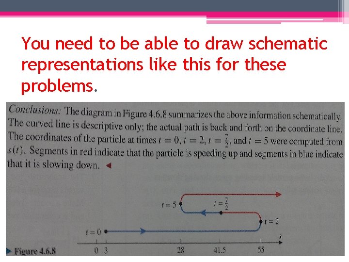
You need to be able to draw schematic representations like this for these problems.

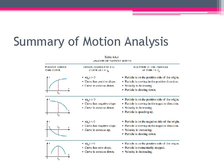
Summary of Motion Analysis

Disneyland with Nephews