Section 4 1 Local Maxima and Minima Applied





- Slides: 34

Section 4. 1 Local Maxima and Minima Applied Calculus , 4/E, Deborah Hughes-Hallett Copyright 2010 by John Wiley and Sons, All Rights Reserved

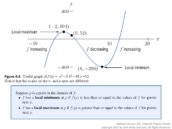
y Figure 4. 2: Useful graph of f (x) = x 3 – 9 x 2 – 48 x +52 Notice that the scales on the x- and y-axes are different. Applied Calculus , 4/E, Deborah Hughes-Hallett Copyright 2010 by John Wiley and Sons, All Rights Reserved

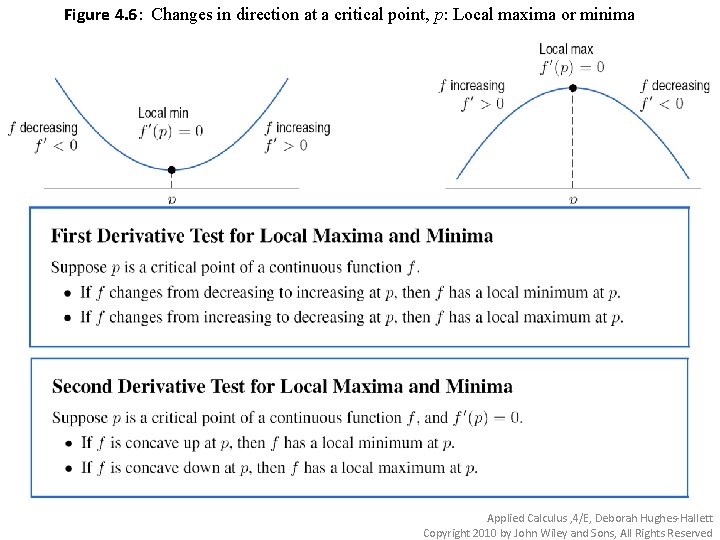
Figure 4. 6: Changes in direction at a critical point, p: Local maxima or minima Applied Calculus , 4/E, Deborah Hughes-Hallett Copyright 2010 by John Wiley and Sons, All Rights Reserved

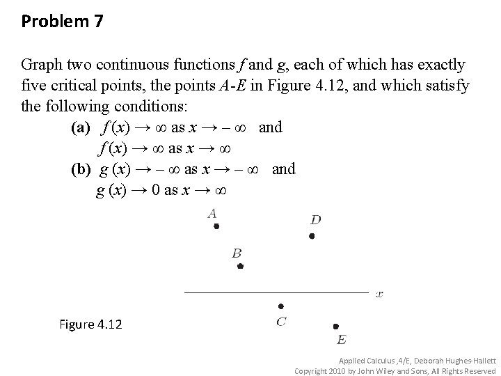
Problem 7 Graph two continuous functions f and g, each of which has exactly five critical points, the points A-E in Figure 4. 12, and which satisfy the following conditions: (a) f (x) → ∞ as x → – ∞ and f (x) → ∞ as x → ∞ (b) g (x) → – ∞ as x → – ∞ and g (x) → 0 as x → ∞ Figure 4. 12 Applied Calculus , 4/E, Deborah Hughes-Hallett Copyright 2010 by John Wiley and Sons, All Rights Reserved

Problem 36 Assume f has a derivative everywhere and just one critical point, at x = 3. In parts (a) – (d), you are given additional conditions. In each case, decide whether x = 3 is a local maximum, a local minimum, or neither. Sketch possible graphs for all four cases. (a) f ‘(1) = 3 and f ‘(5) = – 1 (b) f (x) → ∞ as x → ∞ and as x → – ∞ (c) f (1) = 1, f (2) = 2, f (4) = 4, f (5) = 5 (d) f ‘(2) = – 1, f (3) = 1, f (x) → 3 as x → ∞ Applied Calculus , 4/E, Deborah Hughes-Hallett Copyright 2010 by John Wiley and Sons, All Rights Reserved

Section 4. 2 Periodic Functions Applied Calculus , 4/E, Deborah Hughes-Hallett Copyright 2010 by John Wiley and Sons, All Rights Reserved

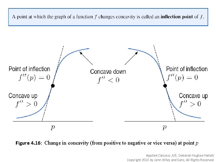
Figure 4. 16: Change in concavity (from positive to negative or vice versa) at point p Applied Calculus , 4/E, Deborah Hughes-Hallett Copyright 2010 by John Wiley and Sons, All Rights Reserved

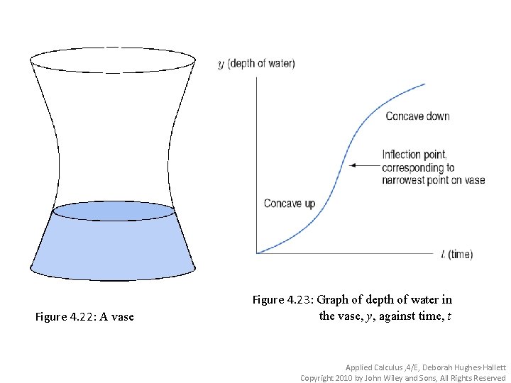
Figure 4. 22: A vase Figure 4. 23: Graph of depth of water in the vase, y, against time, t Applied Calculus , 4/E, Deborah Hughes-Hallett Copyright 2010 by John Wiley and Sons, All Rights Reserved

Section 4. 3 Global Maxima and Minima Applied Calculus , 4/E, Deborah Hughes-Hallett Copyright 2010 by John Wiley and Sons, All Rights Reserved

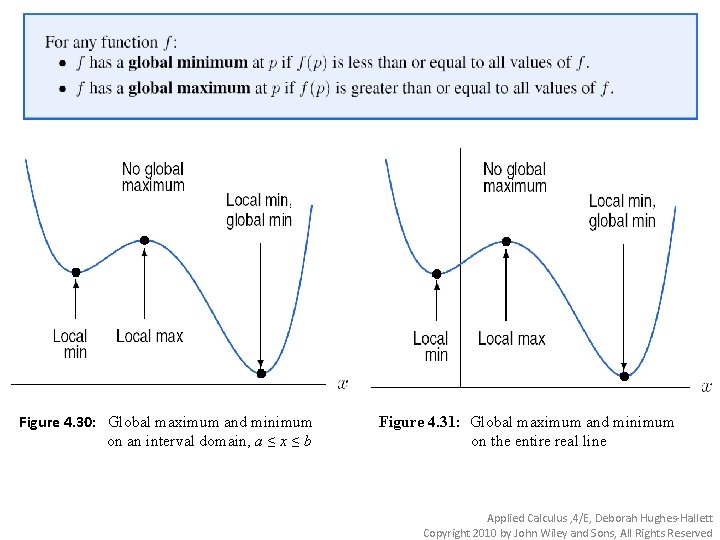
Figure 4. 30: Global maximum and minimum on an interval domain, a ≤ x ≤ b Figure 4. 31: Global maximum and minimum on the entire real line Applied Calculus , 4/E, Deborah Hughes-Hallett Copyright 2010 by John Wiley and Sons, All Rights Reserved

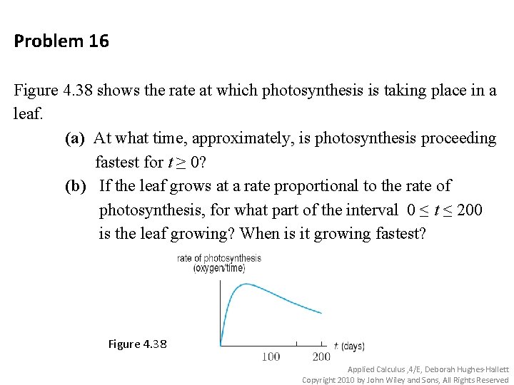
Problem 16 Figure 4. 38 shows the rate at which photosynthesis is taking place in a leaf. (a) At what time, approximately, is photosynthesis proceeding fastest for t ≥ 0? (b) If the leaf grows at a rate proportional to the rate of photosynthesis, for what part of the interval 0 ≤ t ≤ 200 is the leaf growing? When is it growing fastest? Figure 4. 38 Applied Calculus , 4/E, Deborah Hughes-Hallett Copyright 2010 by John Wiley and Sons, All Rights Reserved

Section 4. 4 Profit, Cost, and Revenue Applied Calculus , 4/E, Deborah Hughes-Hallett Copyright 2010 by John Wiley and Sons, All Rights Reserved

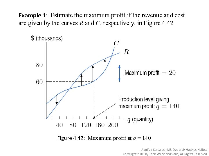
Example 1: Estimate the maximum profit if the revenue and cost are given by the curves R and C, respectively, in Figure 4. 42: Maximum profit at q = 140 Applied Calculus , 4/E, Deborah Hughes-Hallett Copyright 2010 by John Wiley and Sons, All Rights Reserved

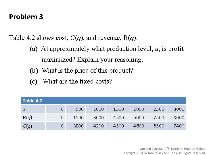
Problem 3 Table 4. 2 shows cost, C(q), and revenue, R(q). (a) At approximately what production level, q, is profit maximized? Explain your reasoning. (b) What is the price of this product? (c) What are the fixed costs? Table 4. 2 q 0 500 1000 1500 2000 2500 3000 R(q) 0 1500 3000 4500 6000 7500 9000 C(q) 0 3800 4200 4500 4800 5500 7400 Applied Calculus , 4/E, Deborah Hughes-Hallett Copyright 2010 by John Wiley and Sons, All Rights Reserved

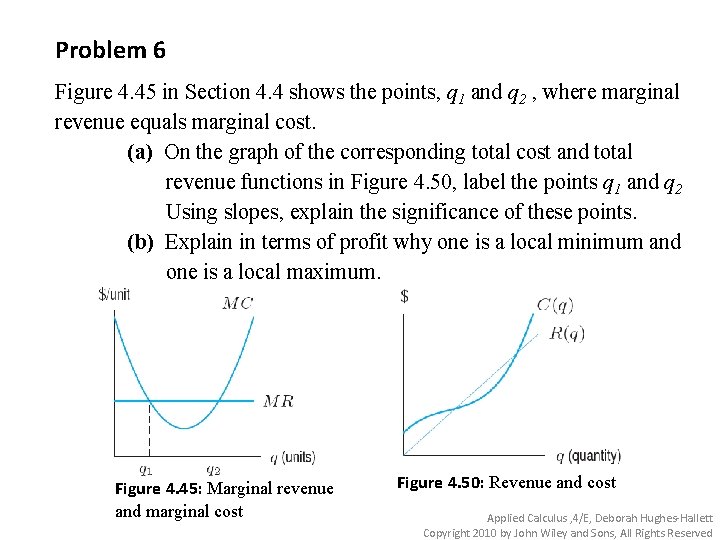
Problem 6 Figure 4. 45 in Section 4. 4 shows the points, q 1 and q 2 , where marginal revenue equals marginal cost. (a) On the graph of the corresponding total cost and total revenue functions in Figure 4. 50, label the points q 1 and q 2 Using slopes, explain the significance of these points. (b) Explain in terms of profit why one is a local minimum and one is a local maximum. Figure 4. 45: Marginal revenue and marginal cost Figure 4. 50: Revenue and cost Applied Calculus , 4/E, Deborah Hughes-Hallett Copyright 2010 by John Wiley and Sons, All Rights Reserved

Section 4. 5 Average Cost Applied Calculus , 4/E, Deborah Hughes-Hallett Copyright 2010 by John Wiley and Sons, All Rights Reserved

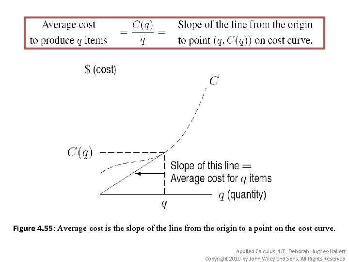
Figure 4. 55: Average cost is the slope of the line from the origin to a point on the cost curve. Applied Calculus , 4/E, Deborah Hughes-Hallett Copyright 2010 by John Wiley and Sons, All Rights Reserved

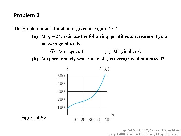
Problem 2 The graph of a cost function is given in Figure 4. 62. (a) At q = 25, estimate the following quantities and represent your answers graphically. (i) Average cost (ii) Marginal cost (b) At approximately what value of q is average cost minimized? Figure 4. 62 Applied Calculus , 4/E, Deborah Hughes-Hallett Copyright 2010 by John Wiley and Sons, All Rights Reserved

Section 4. 6 Elasticity of Demand Applied Calculus , 4/E, Deborah Hughes-Hallett Copyright 2010 by John Wiley and Sons, All Rights Reserved

Is the demand of each of the following products elastic or inelastic? Light bulbs Batteries Furniture Vacation cruise packages Baby formula Gasoline Jewelry New cars Milk Applied Calculus , 4/E, Deborah Hughes-Hallett Copyright 2010 by John Wiley and Sons, All Rights Reserved

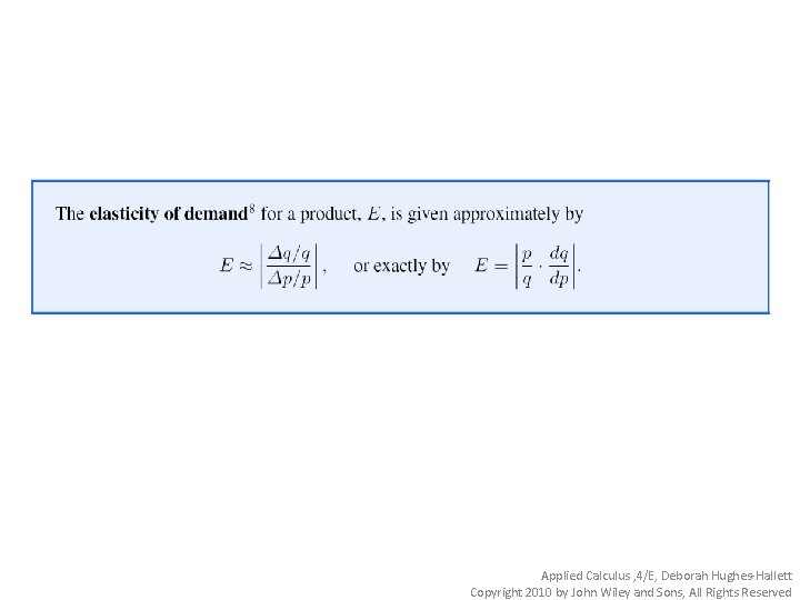
Applied Calculus , 4/E, Deborah Hughes-Hallett Copyright 2010 by John Wiley and Sons, All Rights Reserved

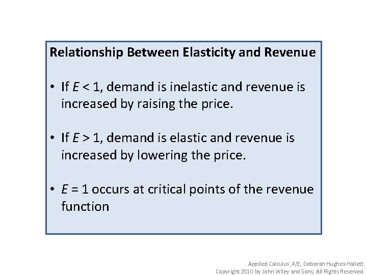
Relationship Between Elasticity and Revenue • If E < 1, demand is inelastic and revenue is increased by raising the price. • If E > 1, demand is elastic and revenue is increased by lowering the price. • E = 1 occurs at critical points of the revenue function Applied Calculus , 4/E, Deborah Hughes-Hallett Copyright 2010 by John Wiley and Sons, All Rights Reserved

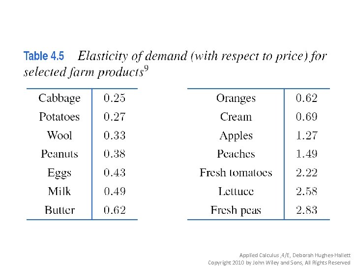
Applied Calculus , 4/E, Deborah Hughes-Hallett Copyright 2010 by John Wiley and Sons, All Rights Reserved

Section 4. 7 Logistic Growth Applied Calculus , 4/E, Deborah Hughes-Hallett Copyright 2010 by John Wiley and Sons, All Rights Reserved

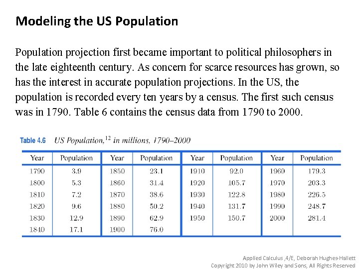
Modeling the US Population projection first became important to political philosophers in the late eighteenth century. As concern for scarce resources has grown, so has the interest in accurate population projections. In the US, the population is recorded every ten years by a census. The first such census was in 1790. Table 6 contains the census data from 1790 to 2000. Applied Calculus , 4/E, Deborah Hughes-Hallett Copyright 2010 by John Wiley and Sons, All Rights Reserved

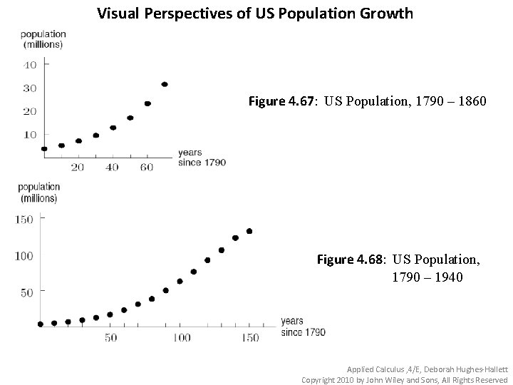
Visual Perspectives of US Population Growth Figure 4. 67: US Population, 1790 – 1860 Figure 4. 68: US Population, 1790 – 1940 Applied Calculus , 4/E, Deborah Hughes-Hallett Copyright 2010 by John Wiley and Sons, All Rights Reserved

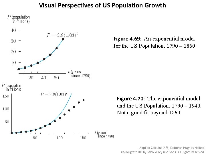
Visual Perspectives of US Population Growth Figure 4. 69: An exponential model for the US Population, 1790 – 1860 Figure 4. 70: The exponential model and the US Population, 1790 – 1940. Not a good fit beyond 1860 Applied Calculus , 4/E, Deborah Hughes-Hallett Copyright 2010 by John Wiley and Sons, All Rights Reserved

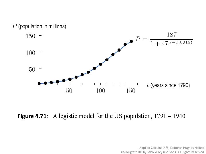
Figure 4. 71: A logistic model for the US population, 1791 – 1940 Applied Calculus , 4/E, Deborah Hughes-Hallett Copyright 2010 by John Wiley and Sons, All Rights Reserved

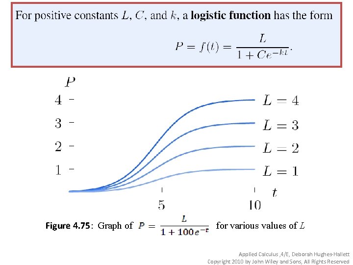
Figure 4. 75: Graph of for various values of L Applied Calculus , 4/E, Deborah Hughes-Hallett Copyright 2010 by John Wiley and Sons, All Rights Reserved

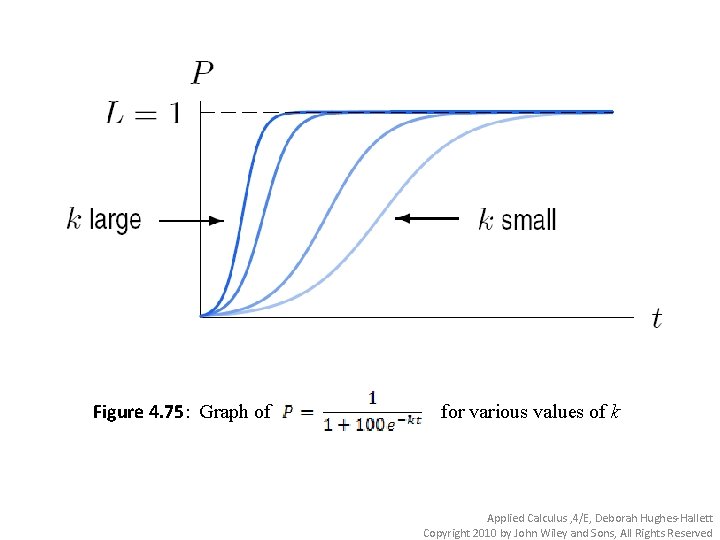
Figure 4. 75: Graph of for various values of k Applied Calculus , 4/E, Deborah Hughes-Hallett Copyright 2010 by John Wiley and Sons, All Rights Reserved

Section 4. 8 The Surge Function and Drug Concentration Applied Calculus , 4/E, Deborah Hughes-Hallett Copyright 2010 by John Wiley and Sons, All Rights Reserved

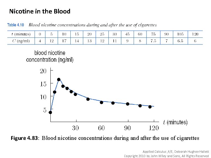
Nicotine in the Blood Figure 4. 83: Blood nicotine concentrations during and after the use of cigarettes Applied Calculus , 4/E, Deborah Hughes-Hallett Copyright 2010 by John Wiley and Sons, All Rights Reserved

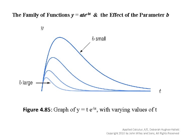
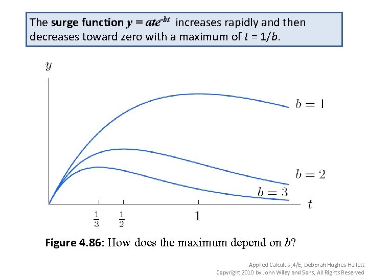
The Family of Functions y = ate-bt & the Effect of the Parameter b Figure 4. 85: Graph of y = t e-bt, with varying values of t Applied Calculus , 4/E, Deborah Hughes-Hallett Copyright 2010 by John Wiley and Sons, All Rights Reserved

The surge function y = ate-bt increases rapidly and then decreases toward zero with a maximum of t = 1/b. Figure 4. 86: How does the maximum depend on b? Applied Calculus , 4/E, Deborah Hughes-Hallett Copyright 2010 by John Wiley and Sons, All Rights Reserved