Section 3 Belief Propagation QA Methods like BP

Section 3: Belief Propagation Q&A Methods like BP and in what sense they work 1

Outline • Do you want to push past the simple NLP models (logistic regression, PCFG, etc. ) that we've all been using for 20 years? • Then this tutorial is extremely practical for you! 1. 2. 3. 4. 5. 6. 7. Models: Factor graphs can express interactions among linguistic structures. Algorithm: BP estimates the global effect of these interactions on each variable, using local computations. Intuitions: What’s going on here? Can we trust BP’s estimates? Fancier Models: Hide a whole grammar and dynamic programming algorithm within a single factor. BP coordinates multiple factors. Tweaked Algorithm: Finish in fewer steps and make the steps faster. Learning: Tune the parameters. Approximately improve the true predictions -- or truly improve the approximate predictions. Software: Build the model you want! 2

Outline • Do you want to push past the simple NLP models (logistic regression, PCFG, etc. ) that we've all been using for 20 years? • Then this tutorial is extremely practical for you! 1. 2. 3. 4. 5. 6. 7. Models: Factor graphs can express interactions among linguistic structures. Algorithm: BP estimates the global effect of these interactions on each variable, using local computations. Intuitions: What’s going on here? Can we trust BP’s estimates? Fancier Models: Hide a whole grammar and dynamic programming algorithm within a single factor. BP coordinates multiple factors. Tweaked Algorithm: Finish in fewer steps and make the steps faster. Learning: Tune the parameters. Approximately improve the true predictions -- or truly improve the approximate predictions. Software: Build the model you want! 3

Q&A Q: Forward-backward is to the Viterbi algorithm as sum-product BP is to _____ ? A: max-product BP 4

Max-product Belief Propagation • Sum-product BP can be used to compute the marginals, pi(Xi) • Max-product BP can be used to compute the most likely assignment, X* = argmax. X p(X) 5

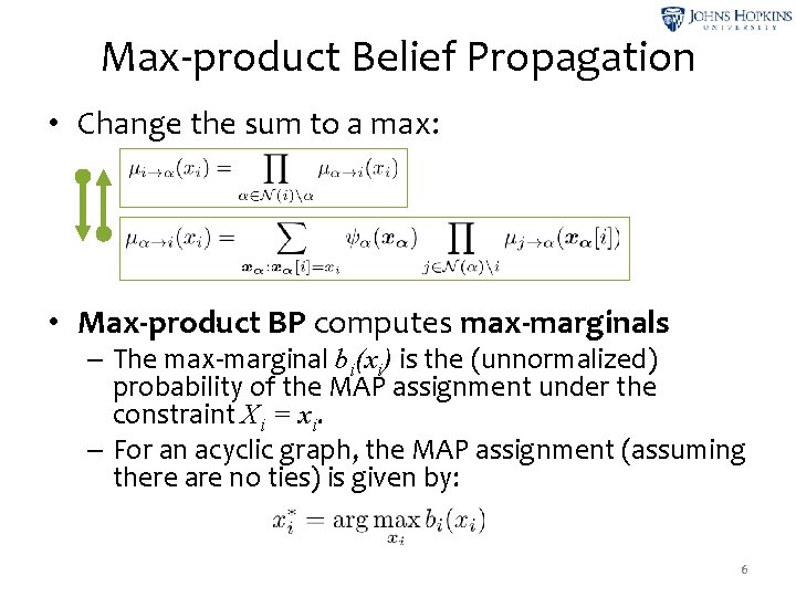
Max-product Belief Propagation • Change the sum to a max: • Max-product BP computes max-marginals – The max-marginal bi(xi) is the (unnormalized) probability of the MAP assignment under the constraint Xi = xi. – For an acyclic graph, the MAP assignment (assuming there are no ties) is given by: 6

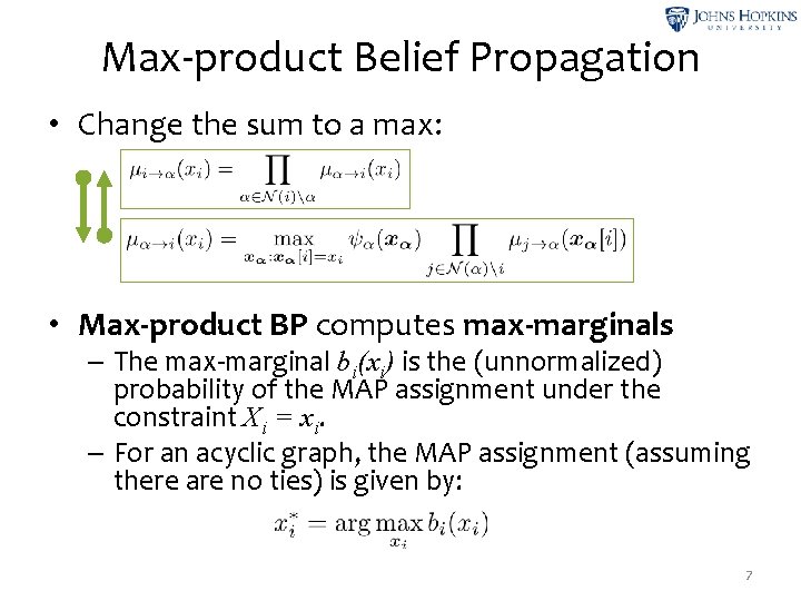
Max-product Belief Propagation • Change the sum to a max: • Max-product BP computes max-marginals – The max-marginal bi(xi) is the (unnormalized) probability of the MAP assignment under the constraint Xi = xi. – For an acyclic graph, the MAP assignment (assuming there are no ties) is given by: 7

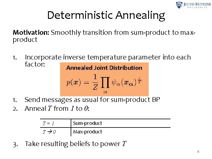
Deterministic Annealing Motivation: Smoothly transition from sum-product to maxproduct 1. Incorporate inverse temperature parameter into each factor: Annealed Joint Distribution 1. Send messages as usual for sum-product BP 2. Anneal T from 1 to 0: T=1 Sum-product T 0 Max-product 3. Take resulting beliefs to power T 8

Q&A Q: This feels like Arc Consistency… Any relation? A: Yes, BP is doing (with probabilities) what people were doing in AI long before. 9

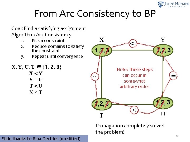
From Arc Consistency to BP Goal: Find a satisfying assignment Algorithm: Arc Consistency 1. 2. 3. Pick a constraint Reduce domains to satisfy the constraint Repeat until convergence X, Y, U, T ∈ {1, 2, 3} X Y Y=U T U X<T X 1, 2, 3 Y 1, 2, 3 Note: These steps can occur in somewhat arbitrary order 1, 2, 3 T = 1, 2, 3 U Propagation completely solved the problem! Slide thanks to Rina Dechter (modified) 10

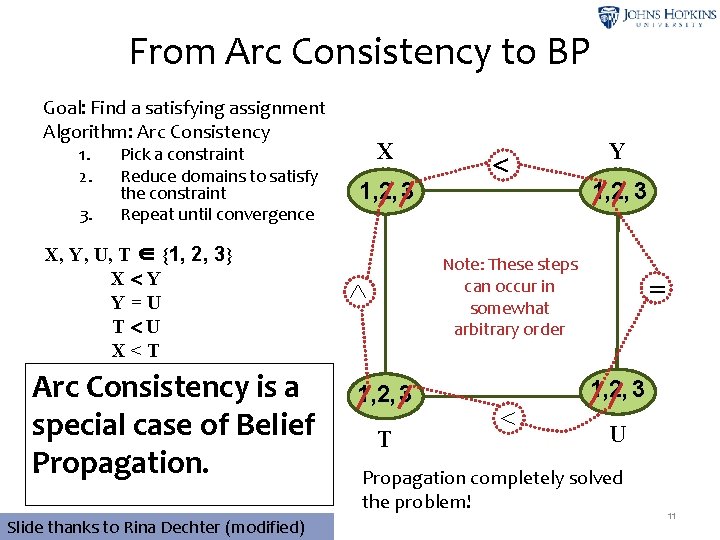
From Arc Consistency to BP Goal: Find a satisfying assignment Algorithm: Arc Consistency 1. 2. 3. Pick a constraint Reduce domains to satisfy the constraint Repeat until convergence X, Y, U, T ∈ {1, 2, 3} X Y Y=U T U X<T Arc Consistency is a special case of Belief Propagation. Slide thanks to Rina Dechter (modified) X 1, 2, 3 Y 1, 2, 3 Note: These steps can occur in somewhat arbitrary order 1, 2, 3 T = 1, 2, 3 U Propagation completely solved the problem! 11

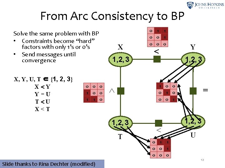
From Arc Consistency to BP Solve the same problem with BP • Constraints become “hard” factors with only 1’s or 0’s • Send messages until convergence X, Y, U, T ∈ {1, 2, 3} X Y Y=U T U X<T 0 0 0 1 1 0 X 1, 2, 3 Y 1, 2, 3 1 0 0 0 1 1, 2, 3 T Slide thanks to Rina Dechter (modified) 0 1 1 0 0 0 = 1, 2, 3 U 12

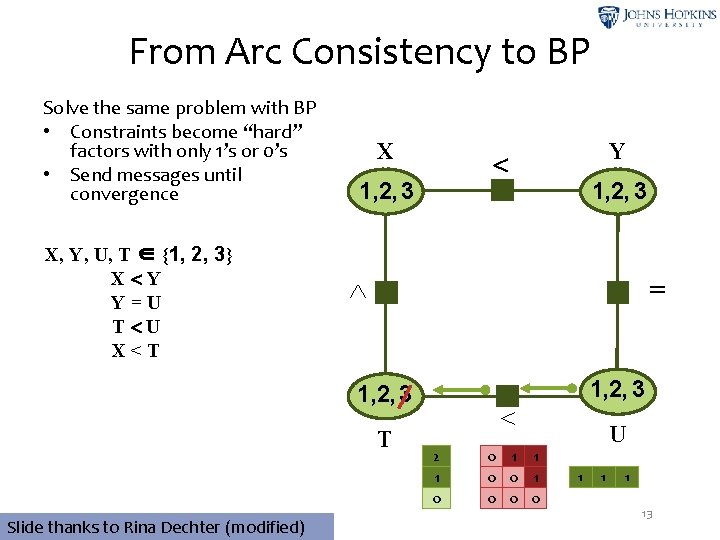
From Arc Consistency to BP Solve the same problem with BP • Constraints become “hard” factors with only 1’s or 0’s • Send messages until convergence X, Y, U, T ∈ {1, 2, 3} X Y Y=U T U X<T X 1, 2, 3 = 1, 2, 3 T Slide thanks to Rina Dechter (modified) Y 1, 2, 3 2 1 0 0 0 U 1 13

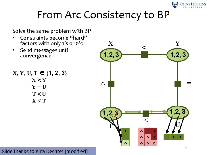
From Arc Consistency to BP Solve the same problem with BP • Constraints become “hard” factors with only 1’s or 0’s • Send messages until convergence X, Y, U, T ∈ {1, 2, 3} X Y Y=U T U X<T X 1, 2, 3 = 1, 2, 3 T Slide thanks to Rina Dechter (modified) Y 1, 2, 3 2 1 0 0 0 U 1 14

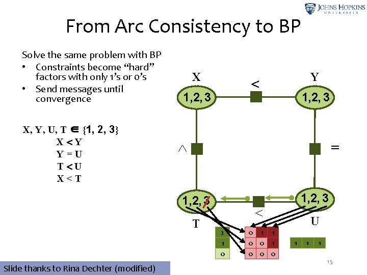
From Arc Consistency to BP Solve the same problem with BP • Constraints become “hard” factors with only 1’s or 0’s • Send messages until convergence X, Y, U, T ∈ {1, 2, 3} X Y Y=U T U X<T X 1, 2, 3 = 1, 2, 3 T Slide thanks to Rina Dechter (modified) Y 1, 2, 3 2 1 0 0 0 U 1 15

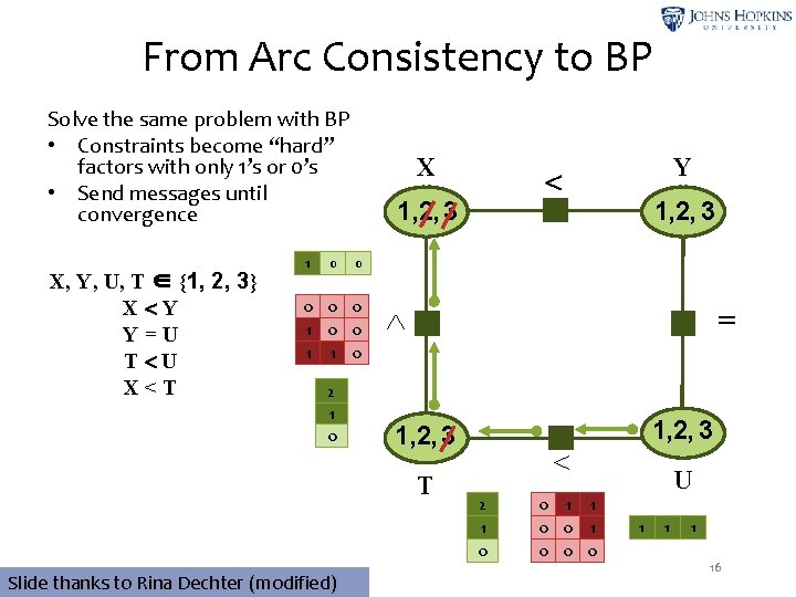
From Arc Consistency to BP Solve the same problem with BP • Constraints become “hard” factors with only 1’s or 0’s • Send messages until convergence X, Y, U, T ∈ {1, 2, 3} X Y Y=U T U X<T 1 0 X 1, 2, 3 = 1, 2, 3 T Slide thanks to Rina Dechter (modified) 1, 2, 3 0 0 1 1 0 2 1 0 Y 1, 2, 3 2 1 0 0 0 U 1 16

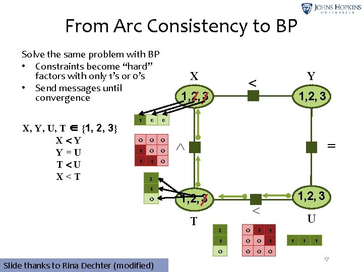
From Arc Consistency to BP Solve the same problem with BP • Constraints become “hard” factors with only 1’s or 0’s • Send messages until convergence X, Y, U, T ∈ {1, 2, 3} X Y Y=U T U X<T 1 0 X 1, 2, 3 = 1, 2, 3 T Slide thanks to Rina Dechter (modified) 1, 2, 3 0 0 1 1 0 2 1 0 Y 1, 2, 3 2 1 0 0 0 U 1 17

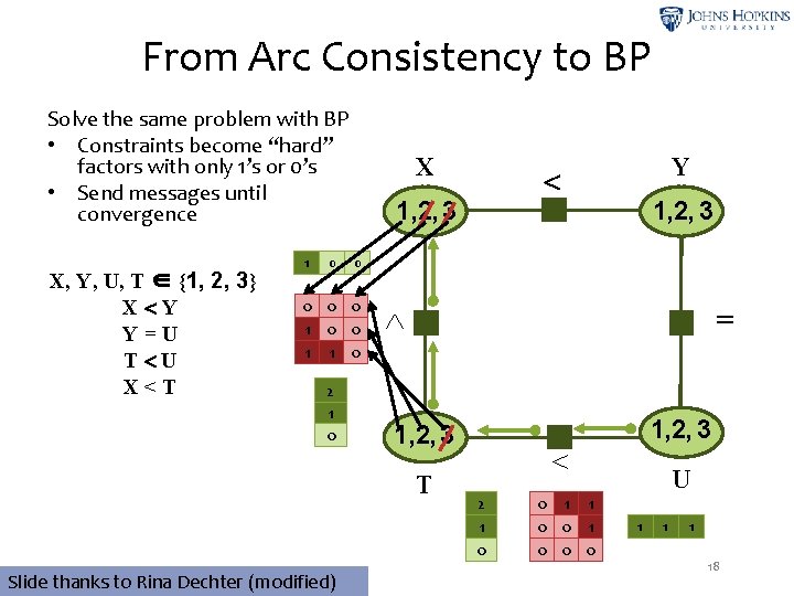
From Arc Consistency to BP Solve the same problem with BP • Constraints become “hard” factors with only 1’s or 0’s • Send messages until convergence X, Y, U, T ∈ {1, 2, 3} X Y Y=U T U X<T 1 0 X 1, 2, 3 = 1, 2, 3 T Slide thanks to Rina Dechter (modified) 1, 2, 3 0 0 1 1 0 2 1 0 Y 1, 2, 3 2 1 0 0 0 U 1 18

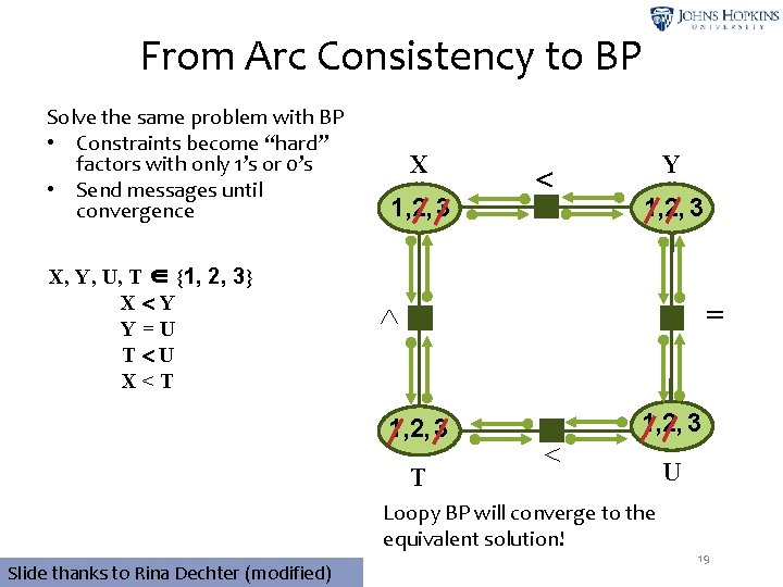
From Arc Consistency to BP Solve the same problem with BP • Constraints become “hard” factors with only 1’s or 0’s • Send messages until convergence X, Y, U, T ∈ {1, 2, 3} X Y Y=U T U X<T X 1, 2, 3 Y 1, 2, 3 = 1, 2, 3 T 1, 2, 3 Loopy BP will converge to the equivalent solution! Slide thanks to Rina Dechter (modified) U 19

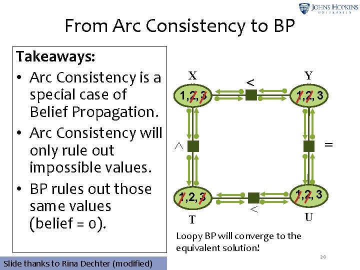
From Arc Consistency to BP Takeaways: X • Arc Consistency is a 1, 2, 3 special case of Belief Propagation. • Arc Consistency will only rule out impossible values. • BP rules out those 1, 2, 3 same values T (belief = 0). Y 1, 2, 3 = 1, 2, 3 Loopy BP will converge to the equivalent solution! Slide thanks to Rina Dechter (modified) U 20

Q&A Q: Is BP totally divorced from sampling? A: Gibbs Sampling is also a kind of message passing algorithm. 21

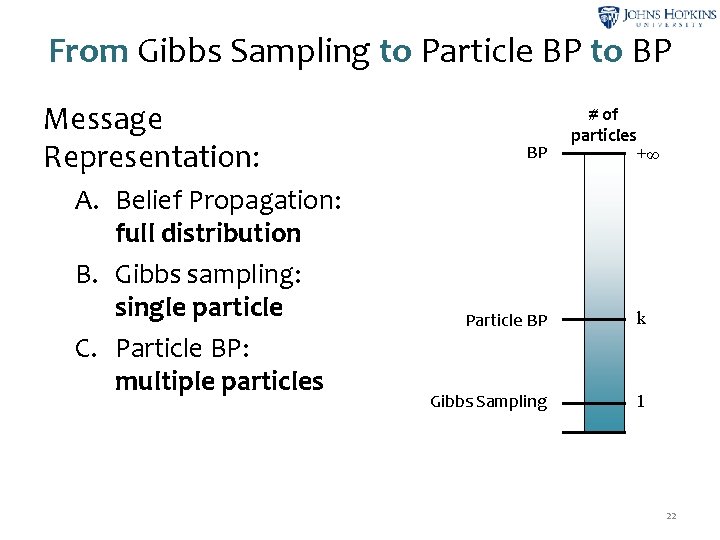
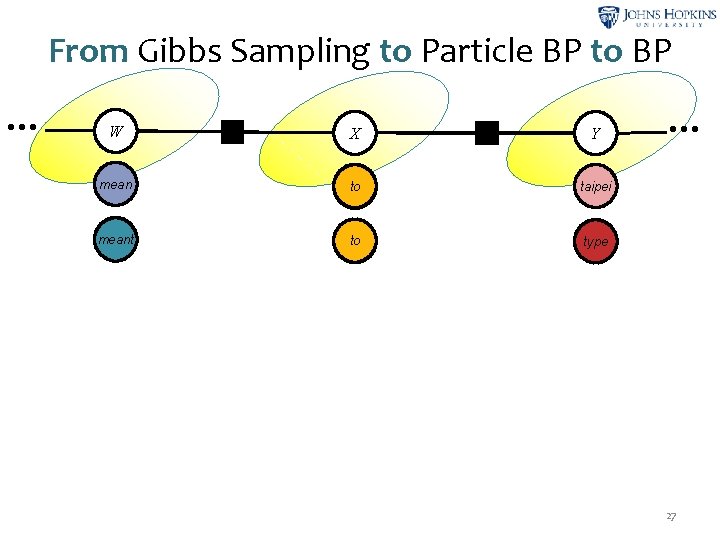
From Gibbs Sampling to Particle BP to BP Message Representation: A. Belief Propagation: full distribution B. Gibbs sampling: single particle C. Particle BP: multiple particles BP # of particles +∞ Particle BP k Gibbs Sampling 1 22

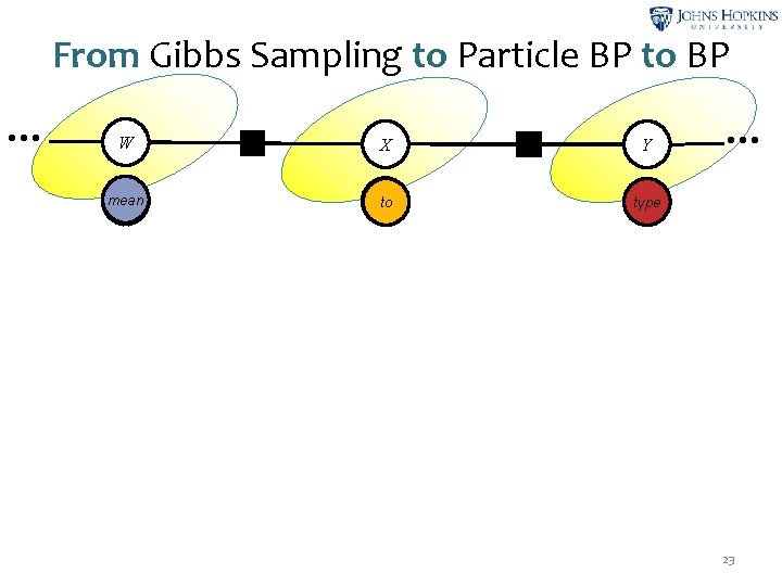
From Gibbs Sampling to Particle BP to BP … W meant ψ2 X too to two ψ3 Y … taipei tight type 23

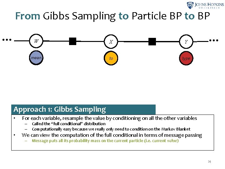
From Gibbs Sampling to Particle BP to BP … W ψ2 meant X ψ3 too to two Y … taipei tight type Approach 1: Gibbs Sampling • For each variable, resample the value by conditioning on all the other variables – Called the “full conditional” distribution – Computationally easy because we really only need to condition on the Markov Blanket • We can view the computation of the full conditional in terms of message passing – Message puts all its probability mass on the current particle (i. e. current value) 24

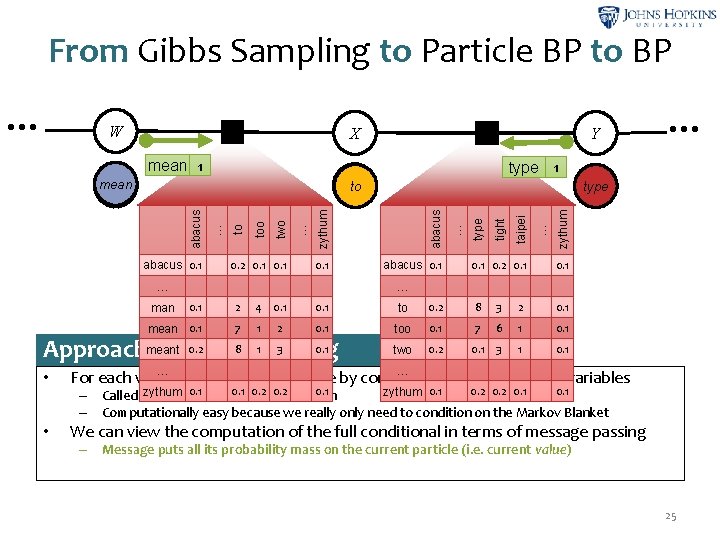
From Gibbs Sampling to Particle BP to BP W ψ2 ψ3 X Y mean 1 meant … 0. 1 0. 2 0. 1 zythum … tight abacus 0. 1 type 0. 1 … abacus taipei tight type zythum 0. 2 0. 1 … two to … abacus too to two abacus 0. 1 … 0. 1 2 4 0. 1 to 0. 2 8 3 2 0. 1 mean 0. 1 7 1 0. 1 too 0. 1 7 6 1 0. 1 two 0. 2 0. 1 3 1 0. 1 man … type 1 taipei … 2 0. 2 8 Sampling 1 3 0. 1 Approachmeant 1: Gibbs • … … For each variable, resample the value by conditioning on all the other variables • We can view the computation of the full conditional in terms of message passing 0. 1 0. 2 distribution 0. 2 0. 1 zythum 0. 1 – Called the “full 0. 1 conditional” – Computationally easy because we really only need to condition on the Markov Blanket – Message puts all its probability mass on the current particle (i. e. current value) 25

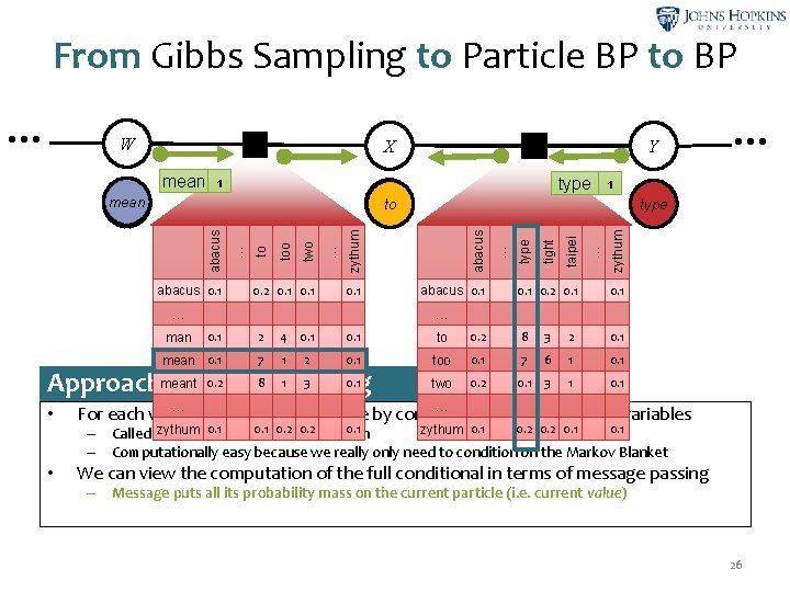
From Gibbs Sampling to Particle BP to BP W ψ2 ψ3 X Y mean 1 meant … 0. 1 0. 2 0. 1 zythum … tight abacus 0. 1 type 0. 1 … abacus taipei tight type zythum 0. 2 0. 1 … two to … abacus too to two abacus 0. 1 … 0. 1 2 4 0. 1 to 0. 2 8 3 2 0. 1 mean 0. 1 7 1 0. 1 too 0. 1 7 6 1 0. 1 two 0. 2 0. 1 3 1 0. 1 man … type 1 taipei … 2 0. 2 8 Sampling 1 3 0. 1 Approachmeant 1: Gibbs • … … For each variable, resample the value by conditioning on all the other variables • We can view the computation of the full conditional in terms of message passing 0. 1 0. 2 distribution 0. 2 0. 1 zythum 0. 1 – Called the “full 0. 1 conditional” – Computationally easy because we really only need to condition on the Markov Blanket – Message puts all its probability mass on the current particle (i. e. current value) 26

From Gibbs Sampling to Particle BP to BP … W ψ2 X ψ3 Y meant mean two to too taipei type man meant to tight too tight type … 27

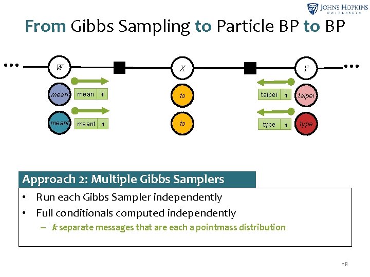
From Gibbs Sampling to Particle BP to BP … W ψ2 X ψ3 Y meant mean 1 two to too taipei 1 taipei type man meant 1 to tight too type 1 tight type … Approach 2: Multiple Gibbs Samplers • Run each Gibbs Sampler independently • Full conditionals computed independently – k separate messages that are each a pointmass distribution 28

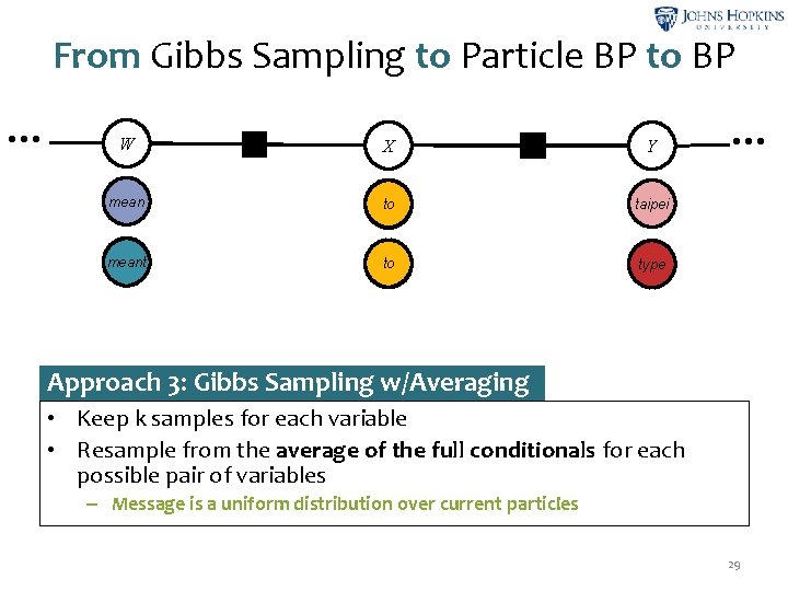
From Gibbs Sampling to Particle BP to BP … W ψ2 X ψ3 Y meant mean two to too taipei type man meant to tight too tight type … Approach 3: Gibbs Sampling w/Averaging • Keep k samples for each variable • Resample from the average of the full conditionals for each possible pair of variables – Message is a uniform distribution over current particles 29

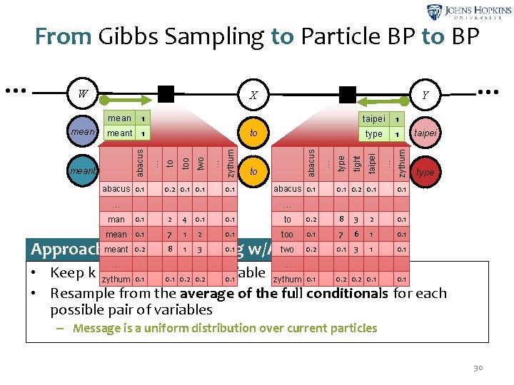
From Gibbs Sampling to Particle BP to BP abacus 0. 1 0. 2 0. 1 … abacus 0. 1 tight type to tight too … abacus zythum … two man meant two to too meant 1 to meant mean taipei 1 type 1 taipei type zythum Y 1 abacus mean ψ3 X tight type 0. 1 0. 2 0. 1 … ψ2 taipei W … … 0. 1 2 4 0. 1 to 0. 2 8 3 2 0. 1 mean 0. 1 7 1 0. 1 too 0. 1 7 6 1 0. 1 3 1 0. 1 man 2 0. 2 8 Sampling 1 3 0. 1 two 0. 2 Approachmeant 3: Gibbs w/Averaging … … … • Keep k samples for each variable 0. 1 0. 2 0. 1 zythum 0. 1 • Resample from the average of the full conditionals for each possible pair of variables – Message is a uniform distribution over current particles 30

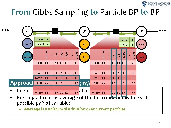
From Gibbs Sampling to Particle BP to BP abacus 0. 1 0. 2 0. 1 … abacus 0. 1 tight type to tight too … abacus zythum … two man meant two to too meant 1 to meant mean taipei 1 type 1 taipei type zythum Y 1 abacus mean ψ3 X tight type 0. 1 0. 2 0. 1 … ψ2 taipei W … … 0. 1 2 4 0. 1 to 0. 2 8 3 2 0. 1 mean 0. 1 7 1 0. 1 too 0. 1 7 6 1 0. 1 3 1 0. 1 man 2 0. 2 8 Sampling 1 3 0. 1 two 0. 2 Approachmeant 3: Gibbs w/Averaging … … … • Keep k samples for each variable 0. 1 0. 2 0. 1 zythum 0. 1 • Resample from the average of the full conditionals for each possible pair of variables – Message is a uniform distribution over current particles 31

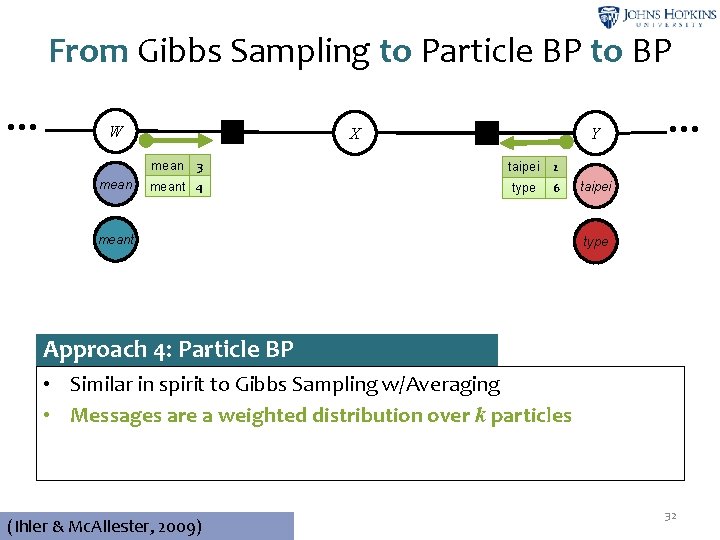
From Gibbs Sampling to Particle BP to BP … W meant mean ψ2 X ψ3 Y mean 3 taipei 2 meant 4 type 6 man meant … taipei type tight type Approach 4: Particle BP • Similar in spirit to Gibbs Sampling w/Averaging • Messages are a weighted distribution over k particles (Ihler & Mc. Allester, 2009) 32

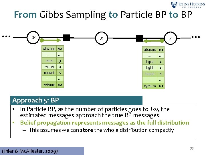
From Gibbs Sampling to Particle BP to BP … W ψ2 abacus 0. 1 X ψ3 Y abacus 0. 1 … … man 3 type 2 mean 4 tight 2 meant 5 taipei 1 … … zythum 0. 1 Approach 5: BP • In Particle BP, as the number of particles goes to +∞, the estimated messages approach the true BP messages • Belief propagation represents messages as the full distribution – This assumes we can store the whole distribution compactly (Ihler & Mc. Allester, 2009) 33

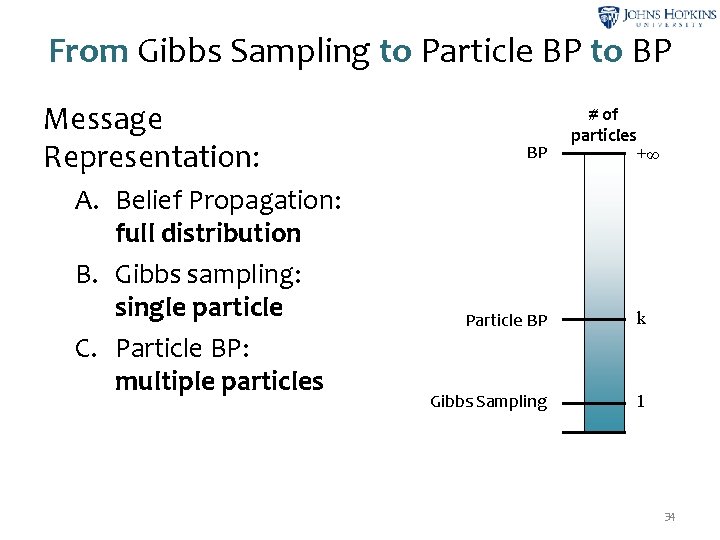
From Gibbs Sampling to Particle BP to BP Message Representation: A. Belief Propagation: full distribution B. Gibbs sampling: single particle C. Particle BP: multiple particles BP # of particles +∞ Particle BP k Gibbs Sampling 1 34

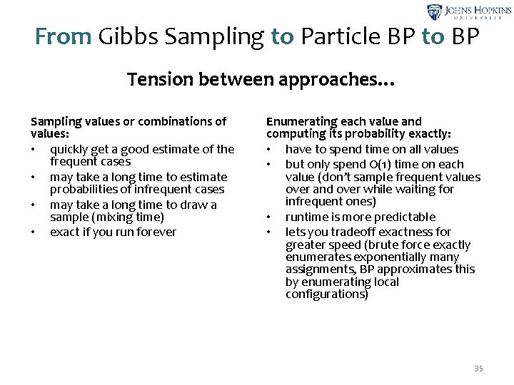
From Gibbs Sampling to Particle BP to BP Tension between approaches… Sampling values or combinations of values: • quickly get a good estimate of the frequent cases • may take a long time to estimate probabilities of infrequent cases • may take a long time to draw a sample (mixing time) • exact if you run forever Enumerating each value and computing its probability exactly: • have to spend time on all values • but only spend O(1) time on each value (don’t sample frequent values over and over while waiting for infrequent ones) • runtime is more predictable • lets you tradeoff exactness for greater speed (brute force exactly enumerates exponentially many assignments, BP approximates this by enumerating local configurations) 35

Background: Convergence When BP is run on a tree-shaped factor graph, the beliefs converge to the marginals of the distribution after two passes. 36

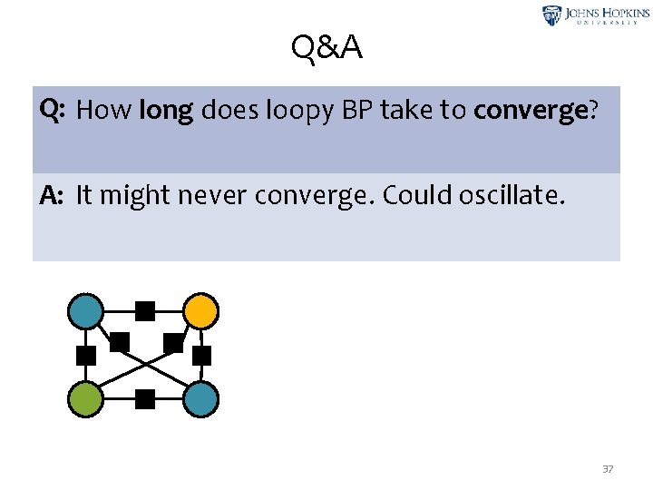
Q&A Q: How long does loopy BP take to converge? A: It might never converge. Could oscillate. ψ2 ψ1 ψ2 37

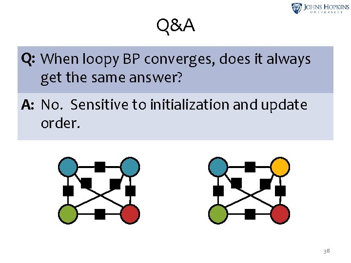
Q&A Q: When loopy BP converges, does it always get the same answer? A: No. Sensitive to initialization and update order. ψ2 ψ1 ψ2 ψ2 ψ1 ψ2 38

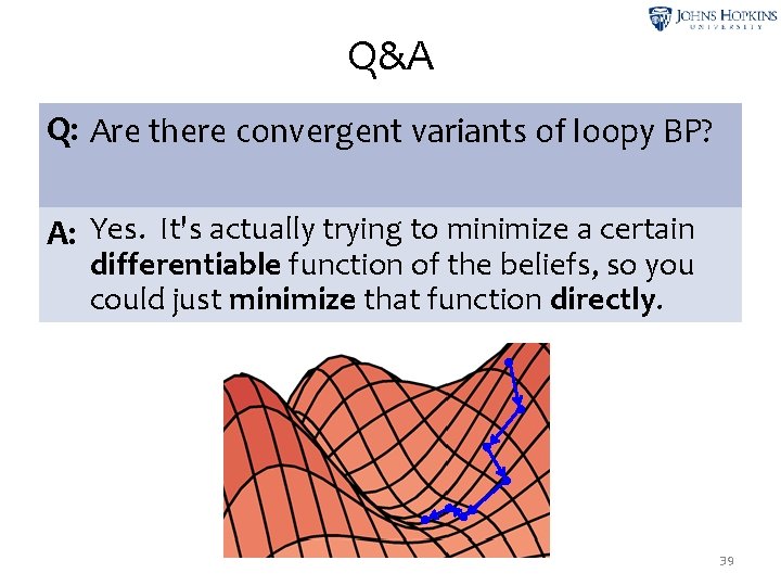
Q&A Q: Are there convergent variants of loopy BP? A: Yes. It's actually trying to minimize a certain differentiable function of the beliefs, so you could just minimize that function directly. 39

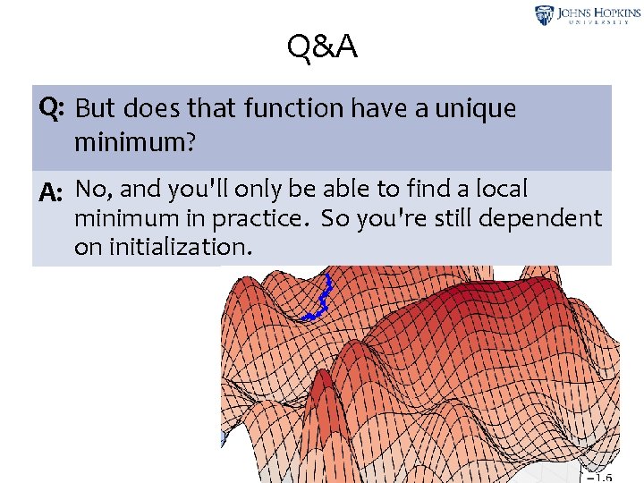
Q&A Q: But does that function have a unique minimum? A: No, and you'll only be able to find a local minimum in practice. So you're still dependent on initialization. 40

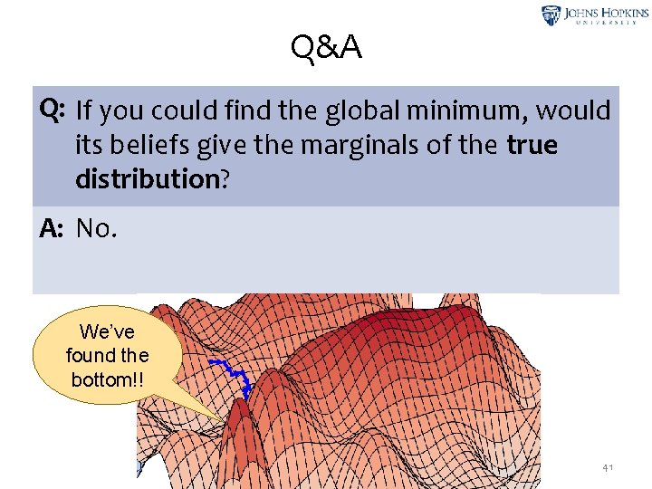
Q&A Q: If you could find the global minimum, would its beliefs give the marginals of the true distribution? A: No. We’ve found the bottom!! 41

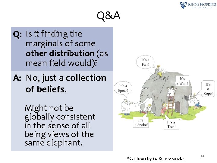
Q&A Q: Is it finding the marginals of some other distribution (as mean field would)? A: No, just a collection of beliefs. Might not be globally consistent in the sense of all being views of the same elephant. *Cartoon by G. Renee Guzlas 42

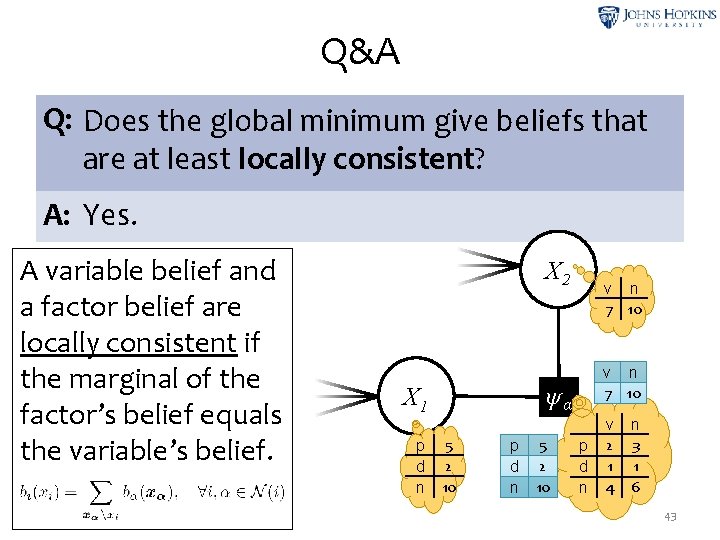
Q&A Q: Does the global minimum give beliefs that are at least locally consistent? A: Yes. A variable belief and a factor belief are locally consistent if the marginal of the factor’s belief equals the variable’s belief. X 2 v n 7 10 ψα X 1 p d n v n 7 10 5 2 10 p d n v 2 1 4 n 3 1 6 43

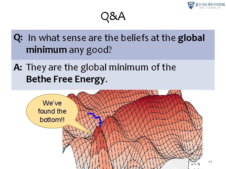
Q&A Q: In what sense are the beliefs at the global minimum any good? A: They are the global minimum of the Bethe Free Energy. We’ve found the bottom!! 44

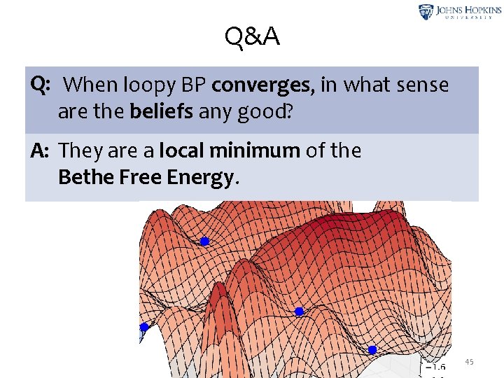
Q&A Q: When loopy BP converges, in what sense are the beliefs any good? A: They are a local minimum of the Bethe Free Energy. 45

Q&A Q: Why would you want to minimize the Bethe Free Energy? A: 1) It’s easy to minimize* because it’s a sum of functions on the individual beliefs. 2) On an acyclic factor graph, it measures KL divergence between beliefs and true marginals, and so is minimized when beliefs = marginals. (For a loopy graph, we close our eyes and hope it still works. ) [*] Though we can’t just minimize each function separately – we need message passing to keep the beliefs locally consistent. 46