Section 10 1 Scatter Plots and Trend Lines

Section 10. 1: Scatter Plots and Trend Lines 1

Objective(s): By following instructions, students will be able to: 1. Describe the relationship between two variables and use it to make predictions. 2

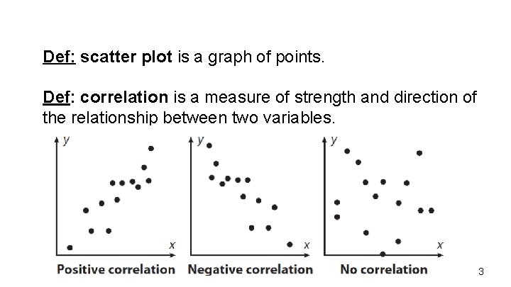
Def: scatter plot is a graph of points. Def: correlation is a measure of strength and direction of the relationship between two variables. 3

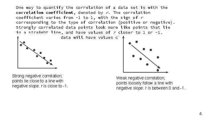
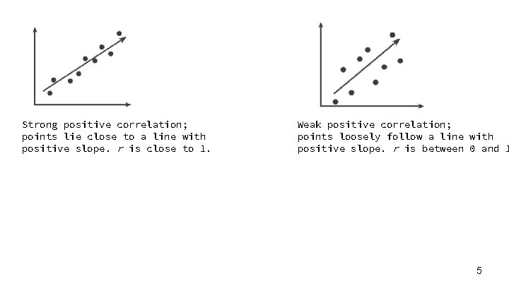
One way to quantify the correlation of a data set is with the correlation coefficient, denoted by r. The correlation coefficient varies from -1 to 1, with the sign of r corresponding to the type of correlation (positive or negative). Strongly correlated data points look more like points that lie in a straight line, and have values of r closer to 1 or -1. Weakly correlated data will have values closer to 0. Strong negative correlation; points lie close to a line with negative slope. r is close to -1. Weak negative correlation; points loosely follow a line with negative slope. r is between 0 and -1. 4

Strong positive correlation; points lie close to a line with positive slope. r is close to 1. Weak positive correlation; points loosely follow a line with positive slope. r is between 0 and 1 5

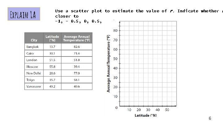
Explain 1 A Use a scatter plot to estimate the value of r. Indicate whether r closer to -1, - 0. 5, 0, 0. 5, or 1. 6

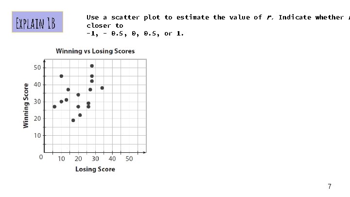
Explain 1 B Use a scatter plot to estimate the value of r. Indicate whether r closer to -1, - 0. 5, 0, 0. 5, or 1. 7

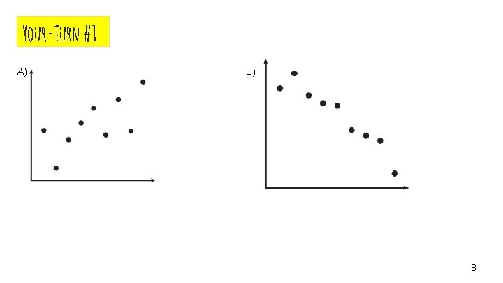
Your-Turn #1 A) B) 8

Def: line of fit is a line through a set of two-variable data that illustrates the correlation. 9

Explain 2 A Determine a line of fit for the data, and write the equation of the line. Go back to the scatter plot of city temperatures and latitudes and add a line of fit. 10

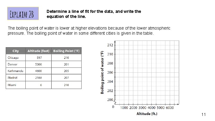
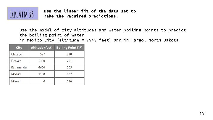
Explain 2 B Determine a line of fit for the data, and write the equation of the line. The boiling point of water is lower at higher elevations because of the lower atmospheric pressure. The boiling point of water in some different cities is given in the table. 11

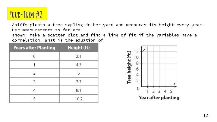
Your-Turn #2 Aoiffe plants a tree sapling in her yard and measures its height every year. Her measurements so far are shown. Make a scatter plot and find a line of fit if the variables have a correlation. What is the equation of your line of fit? 12

Def: interpolation and extrapolation are methods of predicting data values for one variable from another based on the line of fit. 13

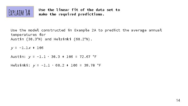
Explain 3 A Use the linear fit of the data set to make the required predictions. Use the model constructed in Example 2 A to predict the average annual temperatures for Austin (30. 3°N) and Helsinki (60. 2°N). y = -1. 1 x + 106 Austin: y = -1. 1 ∙ 30. 3 + 106 = 72. 67 °F Helsinki: y = -1. 1 ∙ 60. 2 + 106 = 39. 78 °F 14

Explain 3 B Use the linear fit of the data set to make the required predictions. Use the model of city altitudes and water boiling points to predict the boiling point of water in Mexico City (altitude = 7943 feet) and in Fargo, North Dakota (altitude = 3000 feet) 15

Read the description of the experiments, identify the two variables and describe whether changing either variable is likely, doubtful, or unclear to a cream changeshop in the otherits variable. The manager of cause an ice studies monthly sales figures and notices a positive correlation between the average air temperature and how much ice cream they sell on any given day. Explain 4 A 16

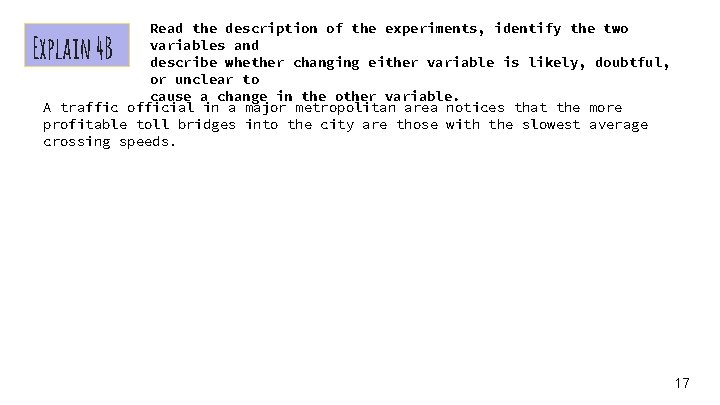
Read the description of the experiments, identify the two variables and describe whether changing either variable is likely, doubtful, or unclear to cause a change in the other variable. A traffic official in a major metropolitan area notices that the more profitable toll bridges into the city are those with the slowest average crossing speeds. Explain 4 B 17

HW: Sec 10. 1 #s 1 -12 ALL, 13 -19 ODD, 21 18