Section 1 3 1 4 NUMERICAL DESCRIPTIVE MEASURES

Section 1. 3 -1. 4 NUMERICAL DESCRIPTIVE MEASURES

Mean The mean is obtained by dividing the sum of all values by the number of values in the data set. Thus,

Example 3 -1 Table 3. 1 lists the total sales (rounded to billions of dollars) of six U. S. companies for 2008.

Table 3. 1 2008 Sales of Six U. S. Companies Find the 2008 mean sales for these six companies.

Example 3 -1: Solution Thus, the mean 2008 sales of these six companies was 228, or $228 billion.

Example 3 -2 The following are the ages (in years) of all eight employees of a small company: 53 32 61 27 39 44 49 57 Find the mean age of these employees.

Example 3 -2: Solution Thus, the mean age of all eight employees of this company is 45. 25 years, or 45 years and 3 months.

Example 3 -3 Table 3. 2 lists the total philanthropic givings (in million dollars) by six companies during 2007.

Example 3 -3 Notice that the charitable contributions made by Wal-Mart are very large compared to those of other companies. Hence, it is an outlier. Show the inclusion of this outlier affects the value of the mean.

Example 3 -3: Solution If we do not include the charitable givings of Wal-Mart (the outlier), the mean of the charitable contributions of the fiver companies is

Example 3 -3: Solution Now, to see the impact of the outlier on the value of the mean, we include the contributions of Wal-Mart and find the mean contributions of the six companies. This mean is

Median

Median Definition The median is the value of the middle term in a data set that has been ranked in increasing order. The calculation of the median consists of the following two steps: 1. Rank the data set in increasing order. 2. Find the middle term. The value of this term is the median.

Example 3 -4 The following data give the prices (in thousands of dollars) of seven houses selected from all houses sold last month in a city. 312 257 421 289 526 374 497 Find the median.

Example 3 -4: Solution First, we rank the given data in increasing order as follows: 257 289 312 374 421 497 526 Since there are seven homes in this data set and the middle term is the fourth term, Thus, the median price of a house is 374.

Example 3 -5 Table 3. 3 gives the 2008 profits (rounded to billions of dollars) of 12 companies selected from all over the world.

Table 3. 3 Profits of 12 Companies for 2008 Find the median of these data.

Example 3 -5: Solution First we rank the given profits as follows: 7 8 9 10 11 12 13 13 14 17 17 45 There are 12 values in this data set. Because there is an even number of values in the data set, the median is given by the average of the two middle values.

Example 3 -5: Solution The two middle values are the sixth and seventh in the foregoing list of data, and these two values are 12 and 13. Thus, the median profit of these 12 companies is $12. 5 billion.

MEASURES OF DISPERSION (VARIBILITY) • Range • Variance and Standard Deviation

Range = Largest value – Smallest Value

Example 3 -11 Table 3. 4 gives the total areas in square miles of the four western South -Central states of the United States. Find the range for this data set.

Table 3. 4

Example 3 -11: Solution Range = Largest value – Smallest Value = 267, 277 – 49, 651 = 217, 626 square miles Thus, the total areas of these four states are spread over a range of 217, 626 square miles.

Definition of Variance and Standard Deviation

An example of deviations Prem Mann, Introductory Statistics, 7/E Copyright © 2010 John Wiley & Sons. All right reserved

Deviations

Variance and Standard Deviation • In general, a lower value of the standard deviation for a data set indicates that the values of that data set are spread over a relatively smaller range around the mean. • In contrast, a large value of the standard deviation for a data set indicates that the values of that data set are spread over a relatively large range around the mean. Prem Mann, Introductory Statistics, 7/E Copyright © 2010 John Wiley & Sons. All right reserved

Example 3 -12 The following table gives the 2008 market values (rounded to billions of dollars) of five international companies. Find the variance and standard deviation for these data. Prem Mann, Introductory Statistics, 7/E Copyright © 2010 John Wiley & Sons. All right reserved

Example 3 -12: Solution Let x denote the 2008 market value of a company. The value of Σx and Σx 2 are calculated in Table 3. 6. Prem Mann, Introductory Statistics, 7/E Copyright © 2010 John Wiley & Sons. All right reserved

Example 3 -12: Solution Thus, the standard deviation of the market values of these five companies is $82. 08 billion. Prem Mann, Introductory Statistics, 7/E Copyright © 2010 John Wiley & Sons. All right reserved

Two Observations 1. The values of the variance and the standard deviation are never negative. 2. The measurement units of variance are always the square of the measurement units of the original data. Prem Mann, Introductory Statistics, 7/E Copyright © 2010 John Wiley & Sons. All right reserved

Population Parameters and Sample Statistics • A numerical measure such as the mean, median, mode, range, variance, or standard deviation calculated for a population data set is called a population parameter, or simply a parameter. • A summary measure calculated for a sample data set is called a sample statistic, or simply a statistic. Prem Mann, Introductory Statistics, 7/E Copyright © 2010 John Wiley & Sons. All right reserved

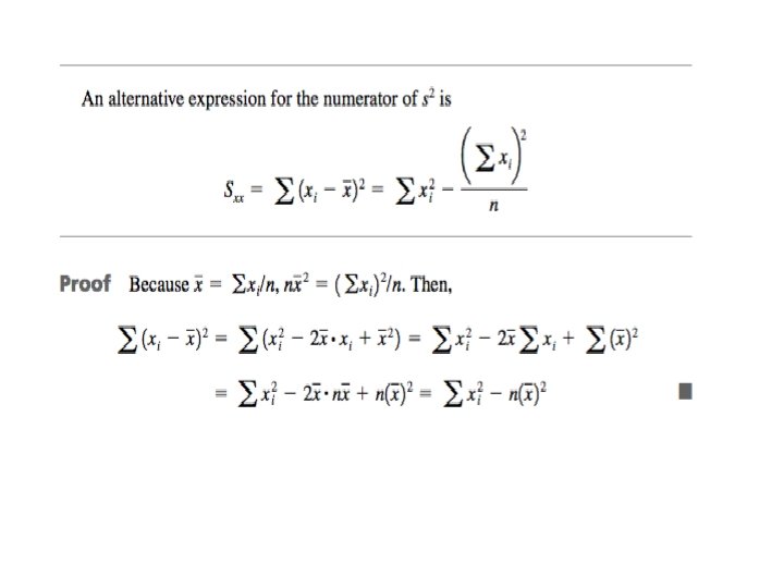
Proposition:

MEASURES OF POSITION • Quartiles and Interquartile Range • Percentiles and Percentile Rank Prem Mann, Introductory Statistics, 7/E Copyright © 2010 John Wiley & Sons. All right reserved

Quartiles and Interquartile Range Quartiles are three summery measures that divide a ranked data set into four equal parts. The second quartile is the same as the median of a data set. The first quartile is the value of the middle term among the observations that are less than the median, and the third quartile is the value of the middle term among the observations that are greater than the median. Prem Mann, Introductory Statistics, 7/E Copyright © 2010 John Wiley & Sons. All right reserved

Figure 3. 11 Quartiles. Prem Mann, Introductory Statistics, 7/E Copyright © 2010 John Wiley & Sons. All right reserved

IQR = Interquartile range = Q 3 – Q 1 Prem Mann, Introductory Statistics, 7/E Copyright © 2010 John Wiley & Sons. All right reserved

Example 3 -20 Refer to Table 3. 3 in Example 3 -5, which gives the 2008 profits (rounded to billions of dollars) of 12 companies selected from all over the world. That table is reproduced below. a) Find the values of the three quartiles. Where does the 2008 profits of Merck & Co fall in relation to these quartiles? b) Find the interquartile range. Prem Mann, Introductory Statistics, 7/E Copyright © 2010 John Wiley & Sons. All right reserved

Table 3. 3 Prem Mann, Introductory Statistics, 7/E Copyright © 2010 John Wiley & Sons. All right reserved

Example 3 -20: Solution a) By looking at the position of $8 billion, which is the 2008 profit of Merck & Co, we can state that this value lies in the bottom 25% of the profits for 2008. Prem Mann, Introductory Statistics, 7/E Copyright © 2010 John Wiley & Sons. All right reserved

Example 3 -20: Solution b) IQR = Interquartile range = Q 3 – Q 1 = 15. 5 – 9. 5 = $6 billion Prem Mann, Introductory Statistics, 7/E Copyright © 2010 John Wiley & Sons. All right reserved

Example 3 -21 The following are the ages (in years) of nine employees of an insurance company: 47 28 39 51 33 37 59 24 33 a) Find the values of the three quartiles. Where does the age of 28 fall in relation to the ages of the employees? b) Find the interquartile range. Prem Mann, Introductory Statistics, 7/E Copyright © 2010 John Wiley & Sons. All right reserved

Example 3 -21: Solution a) Values less than the median Values greater than the median The age of 28 falls in the lowest 25% of the ages. Prem Mann, Introductory Statistics, 7/E Copyright © 2010 John Wiley & Sons. All right reserved

Example 3 -21: Solution b) IQR = Interquartile range = Q 3 – Q 1 = 49 – 30. 5 = 18. 5 years Prem Mann, Introductory Statistics, 7/E Copyright © 2010 John Wiley & Sons. All right reserved

BOX-AND-WHISKER PLOT Definition A plot that shows the center, spread, and skewness of a data set. It is constructed by drawing a box and two whiskers that use the median, the first quartile, the third quartile, and the smallest and the largest values in the data set between the lower and the upper inner fences. Prem Mann, Introductory Statistics, 7/E Copyright © 2010 John Wiley & Sons. All right reserved

Example 3 -24 The following data are the incomes (in thousands of dollars) for a sample of 12 households. 75 69 84 112 74 104 81 90 94 144 79 98 Construct a box-and-whisker plot for these data. Prem Mann, Introductory Statistics, 7/E Copyright © 2010 John Wiley & Sons. All right reserved

Example 3 -24: Solution Step 1. 69 74 75 79 81 84 90 94 98 104 112 144 Median = (84 + 90) / 2 = 87 Q 1 = (75 + 79) / 2 = 77 Q 3 = (98 + 104) / 2 = 101 IQR = Q 3 – Q 1 = 101 – 77 = 24 Prem Mann, Introductory Statistics, 7/E Copyright © 2010 John Wiley & Sons. All right reserved

Example 3 -24: Solution Step 2. 1. 5 x IQR = 1. 5 x 24 = 36 Lower inner fence = Q 1 – 36 = 77 – 36 = 41 Upper inner fence = Q 3 + 36 = 101 + 36 = 137 Prem Mann, Introductory Statistics, 7/E Copyright © 2010 John Wiley & Sons. All right reserved

Example 3 -24: Solution Step 3. Smallest value within the two inner fences = 69 Largest value within the two inner fences = 112 Prem Mann, Introductory Statistics, 7/E Copyright © 2010 John Wiley & Sons. All right reserved

Example 3 -24: Solution Step 4. Figure 3. 13 Prem Mann, Introductory Statistics, 7/E Copyright © 2010 John Wiley & Sons. All right reserved

Example 3 -24: Solution Step 5. Figure 3. 14 Prem Mann, Introductory Statistics, 7/E Copyright © 2010 John Wiley & Sons. All right reserved

Comparative Boxplots In recent years, some evidence suggests that high indoor radon concentration may be linked to the development of childhood cancers, but many health professionals re- main unconvinced. The article “Indoor Radon and Childhood Cancer” (Lancet, 1991: 1537– 1538) presented the accompanying data on radon concentration (Bq/m 3) in two different samples of houses. The first sample consisted of houses in which a child diagnosed with cancer had been residing. Houses in the second sample had no recorded cases of childhood cancer.

Stem-leaf display of data

Numerical summary quantities fs denotes IQR

Comparative Boxplots

Empirical Cumulative Distribution (ECDF) Empirical Cumulative Distribution Function (ECDF): where n represents the sample size.

Example 3 -23 Refer to the data on 2008 profits for 12 companies given in Example 3 -20. Find the ECDF value at $14 billion profit of Petrobras. Give a brief interpretation of value.

Example 3 -23: Solution The data on revenues arranged in increasing order is as follows: 7 8 9 10 11 12 13 13 14 17 17 45 ecdf (7) = 1/12 = 0. 083 ecdf (8) = 2/12 = 0. 167 ecdf (13) = 8/12 = 0. 667

ECDF of 1, 2, 3, 4, 5, and Quantiles

ECDF of 1, 2, …, 20 and Quantiles

A Definition of Quantile and Percentile The kth percentile or k% quantile is defined: where n represents the sample size.

Example 3 -22 Refer to the data on 2008 profits for 12 companies given in Example 3 -20. Find the value of the 42 nd percentile. Give a brief interpretation of the 42 nd percentile. Prem Mann, Introductory Statistics, 7/E Copyright © 2010 John Wiley & Sons. All right reserved

Example 3 -22: Solution The data arranged in increasing order as follows: 7 8 9 10 11 12 13 13 14 17 17 45 The position of the 42 nd percentile is Prem Mann, Introductory Statistics, 7/E Copyright © 2010 John Wiley & Sons. All right reserved

Example 3 -22: Solution The value of the 5. 04 th term can be approximated by the value of the fifth term in the ranked data. Therefore, Q 0. 42 = 42 nd percentile = 11 Thus, approximately 42% of these 12 companies had 2008 profits less than or equal to $11 billion. Prem Mann, Introductory Statistics, 7/E Copyright © 2010 John Wiley & Sons. All right reserved