Sect 5 4 Eigenvalues of I Principal Axis

Sect 5. 4: Eigenvalues of I & Principal Axis Transformation • Definition of inertia tensor (continuous body): Ijk ∫Vρ(r)[r 2δjk - xjxk]d. V – Clearly, Ijk is symmetric: Ijk = Ikj Out of the 9 elements Ijk only 6 are independent. Ijk depend on the location of the origin of the body axes set & on the orientation of the body axes with respect to the body. • Symmetry There exists a set of coordinates Principal Axes in which the tensor Ijk is diagonal with 3 Principal Values I 1, I 2, I 3. In this system, the angular momentum: the KE L = I ω becomes: L 1 = I 1ω1, L 2 = I 2ω2, L 3 = I 3ω3. T = (½)ω I ω becomes: T = (½)I 1(ω1)2 + (½)I 2(ω2)2 + (½)I 3(ω3)2

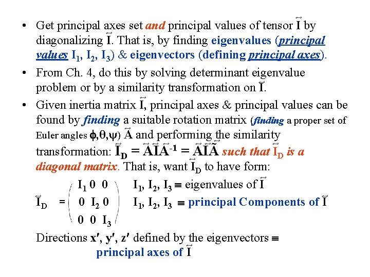
• Get principal axes set and principal values of tensor I by diagonalizing I. That is, by finding eigenvalues (principal values I 1, I 2, I 3) & eigenvectors (defining principal axes). • From Ch. 4, do this by solving determinant eigenvalue problem or by a similarity transformation on I. • Given inertia matrix I, principal axes & principal values can be found by finding a suitable rotation matrix (finding a proper set of Euler angles , θ, ψ) A and performing the similarity transformation: ID = AIA-1 = AIÃ such that ID is a diagonal matrix. That is, want ID to have form: I 1 0 0 I 1, I 2, I 3 eigenvalues of I ID = 0 I 2 0 I 1, I 2, I 3 principal Components of I 0 0 I 3 Directions x , y , z defined by the eigenvectors principal axes of I

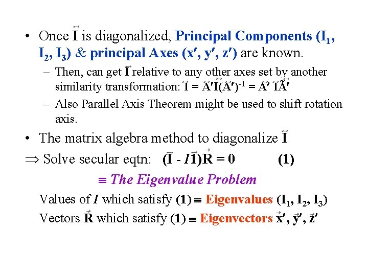
• Once I is diagonalized, Principal Components (I 1, I 2, I 3) & principal Axes (x , y , z ) are known. – Then, can get I relative to any other axes set by another similarity transformation: I = A I(A )-1 = A IÃ – Also Parallel Axis Theorem might be used to shift rotation axis. • The matrix algebra method to diagonalize I Solve secular eqtn: (I - I 1)R = 0 (1) The Eigenvalue Problem Values of I which satisfy (1) Eigenvalues (I 1, I 2, I 3) Vectors R which satisfy (1) Eigenvectors x , y , z

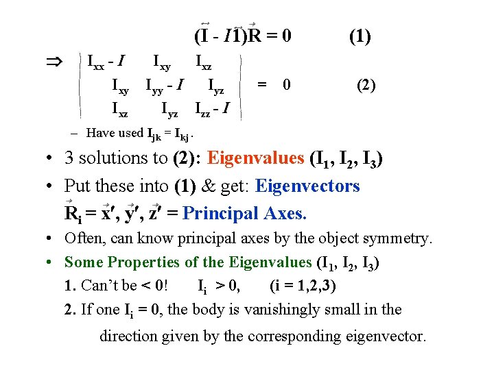
(I - I 1)R = 0 Ixx - I Ixy Ixz Ixy Iyy - I Iyz Ixz Iyz Izz - I = 0 (1) (2) – Have used Ijk = Ikj. • 3 solutions to (2): Eigenvalues (I 1, I 2, I 3) • Put these into (1) & get: Eigenvectors Ri = x , y , z = Principal Axes. • Often, can know principal axes by the object symmetry. • Some Properties of the Eigenvalues (I 1, I 2, I 3) 1. Can’t be < 0! Ii > 0, (i = 1, 2, 3) 2. If one Ii = 0, the body is vanishingly small in the direction given by the corresponding eigenvector.

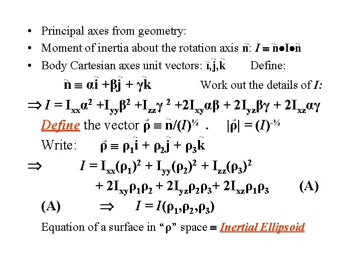
• Principal axes from geometry: • Moment of inertia about the rotation axis n: I n I n • Body Cartesian axes unit vectors: i, j, k Define: n αi +βj + γk Work out the details of I: I = Ixxα 2 +Iyyβ 2 +Izzγ 2 +2 Ixyαβ + 2 Iyzβγ + 2 Ixzαγ Define the vector ρ n/(I)½. |ρ| = (I)-½ Write: ρ ρ1 i + ρ2 j + ρ3 k I = Ixx(ρ1)2 + Iyy(ρ2)2 + Izz(ρ3)2 + 2 Ixyρ1ρ2 + 2 Iyzρ2ρ3+ 2 Ixzρ1ρ3 (A) I = I(ρ1, ρ2, ρ3) Equation of a surface in “ρ” space Inertial Ellipsoid

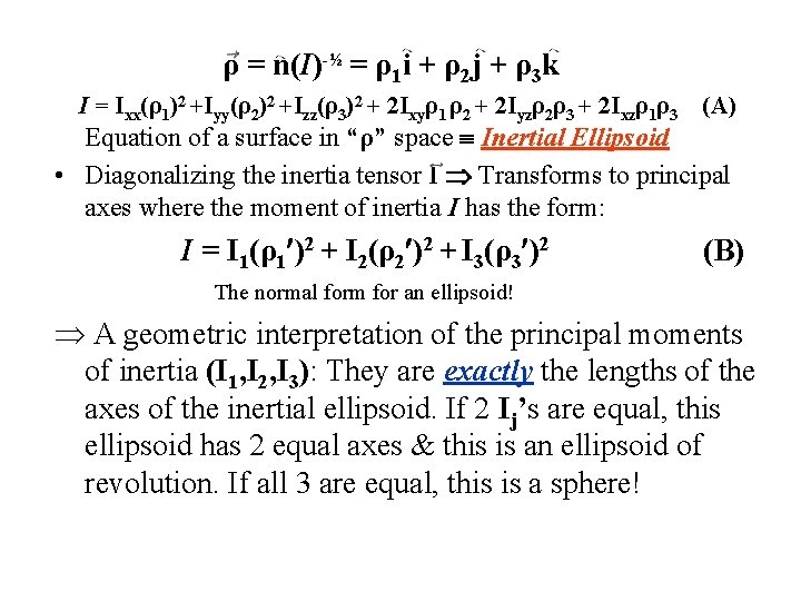
ρ = n(I)-½ = ρ1 i + ρ2 j + ρ3 k I = Ixx(ρ1)2 +Iyy(ρ2)2 +Izz(ρ3)2 + 2 Ixyρ1 ρ2 + 2 Iyzρ2ρ3 + 2 Ixzρ1ρ3 (A) Equation of a surface in “ρ” space Inertial Ellipsoid • Diagonalizing the inertia tensor I Transforms to principal axes where the moment of inertia I has the form: I = I 1(ρ1 )2 + I 2(ρ2 )2 + I 3(ρ3 )2 (B) The normal form for an ellipsoid! A geometric interpretation of the principal moments of inertia (I 1, I 2, I 3): They are exactly the lengths of the axes of the inertial ellipsoid. If 2 Ij’s are equal, this ellipsoid has 2 equal axes & this is an ellipsoid of revolution. If all 3 are equal, this is a sphere!

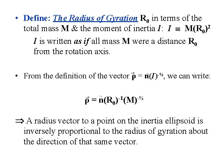
• Define: The Radius of Gyration R 0 in terms of the total mass M & the moment of inertia I: I M(R 0)2 I is written as if all mass M were a distance R 0 from the rotation axis. • From the definition of the vector ρ = n(I)-½, we can write: ρ = n(R 0)-1(M)-½ A radius vector to a point on the inertia ellipsoid is inversely proportional to the radius of gyration about the direction of that same vector.

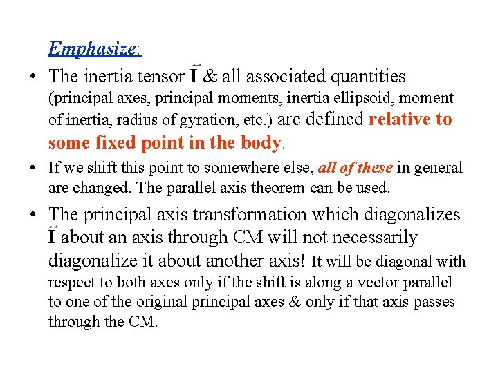
Emphasize: • The inertia tensor I & all associated quantities (principal axes, principal moments, inertia ellipsoid, moment of inertia, radius of gyration, etc. ) are defined relative to some fixed point in the body. • If we shift this point to somewhere else, all of these in general are changed. The parallel axis theorem can be used. • The principal axis transformation which diagonalizes I about an axis through CM will not necessarily diagonalize it about another axis! It will be diagonal with respect to both axes only if the shift is along a vector parallel to one of the original principal axes & only if that axis passes through the CM.

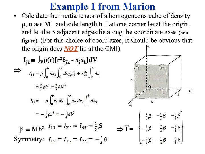
Example 1 from Marion • Calculate the inertia tensor of a homogeneous cube of density ρ, mass M, and side length b. Let one corner be at the origin, and let the 3 adjacent edges lie along the coordinate axes (see figure). (For this choice of coord axes, it should be obvious that the origin does NOT lie at the CM!) Ijk ∫Vρ(r)[r 2δjk - xjxk]d. V β Mb 2 Symmetry: I=

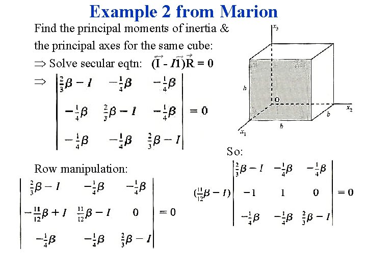
Example 2 from Marion Find the principal moments of inertia & the principal axes for the same cube: Solve secular eqtn: (I - I 1)R = 0 So: Row manipulation:

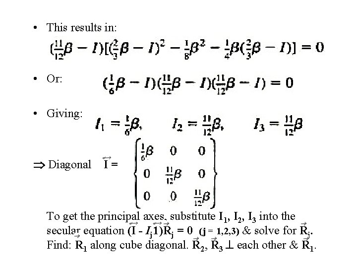
• This results in: • Or: • Giving: Diagonal I= To get the principal axes, substitute I 1, I 2, I 3 into the secular equation (I - Ij 1)Rj = 0 (j = 1, 2, 3) & solve for Rj. Find: R 1 along cube diagonal. R 2, R 3 each other & R 1.

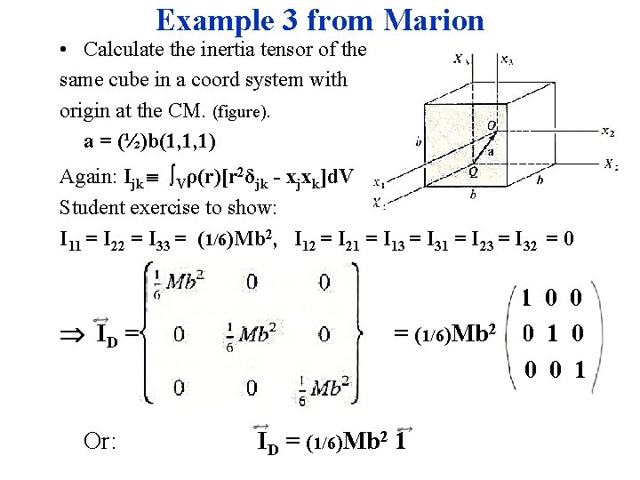
Example 3 from Marion • Calculate the inertia tensor of the same cube in a coord system with origin at the CM. (figure). a = (½)b(1, 1, 1) Again: Ijk ∫Vρ(r)[r 2δjk - xjxk]d. V Student exercise to show: I 11 = I 22 = I 33 = (1/6)Mb 2, I 12 = I 21 = I 13 = I 31 = I 23 = I 32 = 0 ID = Or: = (1/6)Mb 2 ID = (1/6)Mb 2 1 1 0 0 0 1

Sect 5. 5: Solving Rigid Body Problems; The Euler Equations • We now have the tools to solve rigid body dynamics problems. Usually assume holonomic constraints. If not (like rolling friction) need to use special methods. • Usually start by seeking a reference point in the body such that the problem can be split into pure translational + pure rotational parts. • If one point in the body is fixed, then obviously all that is needed is to treat the dynamics of the rotation about that point. • If one point is not fixed, it is most useful to choose the reference point in the body to be the CM.

• We have already seen that, for case where the reference point is the CM, the KE splits into KE of translation of CM + KE of rotation about an axis through the CM: • We had: T = Ttrans + Trot – – 1 st term = Ttrans = (½)Mv 2 Translational KE of the CM 2 nd term = Trot = (½)∑imi(vi)2. Rotational KE about CM We’ve written second term as: Trot = (½)ω I ω For n unit vector along the rotation axis: Trot = (½)ω2 n I n (½) Iω2 • So: T = (½)Mv 2 + (½)Iω2 • For all problems considered here, we can make a similar division for the PE: V = Vtrans + Vrot Lagrangian similarly divides: L = Ltrans + Lrot

• More generally (Goldstein notation): L = Ltrans + Lrot = Lc(qc, qc) + Lb(qb, qb) Lc = CM Lagrangian, qc = generalized coordinates & velocities of the CM. Lb = Body Lagrangian, qb = generalized coordinates & velocities of body (rotation). • Can use either Newtonian or Lagrangian methods, of course. In either case, often convenient to work in the principal axes system so that the rotational KE takes the simple form: Trot = (½)I 1(ω1)2 + (½)I 2(ω2)2 + (½)I 3(ω3)2 • The most convenient generalized coordinates to use are the Euler angles: , θ, ψ. They are cumbersome, but useable. • If the motion is confined to 2 dimensions (the rotation axis is fixed in direction), then only 1 angle describes motion!

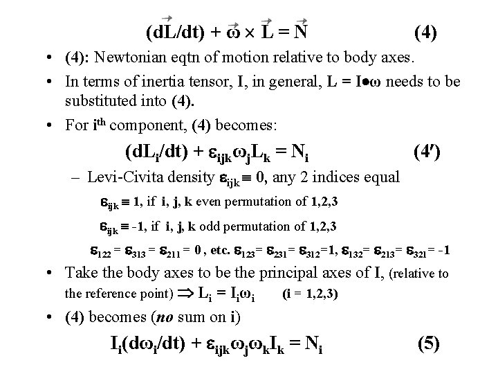
• Follow Goldstein & start with the Newtonian approach to describe the rotational motion about an axis through a fixed point (like the CM): • Consider either an inertial frame with the origin at a fixed point in body or a space axes system with CM as the origin. • In this case, a Ch. 1 result is: (d. L/dt)s = N (1) Newton’s 2 nd Law (rotational motion): Time derivative of the total angular momentum L (taken with respect to the space axes) is equal to the total external torque N. • Make use of the Ch. 4 result relating the time derivatives in the space & body axes (angular velocity ω): (d/dt)s = (d/dt)b + ω (2) (d. L/dt)s = (d. L/dt)b + ω L (3) • Equating (1) & (3) & dropping the “body” subscript (which is understood in what follows) gives:

(d. L/dt) + ω L = N (4) • (4): Newtonian eqtn of motion relative to body axes. • In terms of inertia tensor, I, in general, L = I ω needs to be substituted into (4). • For ith component, (4) becomes: (d. Li/dt) + ijkωj. Lk = Ni (4 ) – Levi-Civita density ijk 0, any 2 indices equal ijk 1, if i, j, k even permutation of 1, 2, 3 ijk -1, if i, j, k odd permutation of 1, 2, 3 122 = 313 = 211 = 0 , etc. 123= 231= 312=1, 132= 213= 321= -1 • Take the body axes to be the principal axes of I, (relative to the reference point) Li = Iiωi (i = 1, 2, 3) • (4) becomes (no sum on i) Ii(dωi/dt) + ijkωjωk. Ik = Ni (5)

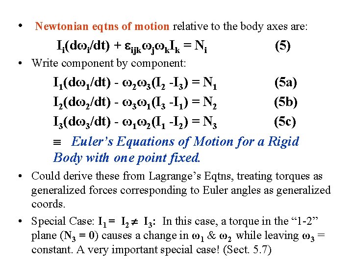
• Newtonian eqtns of motion relative to the body axes are: Ii(dωi/dt) + ijkωjωk. Ik = Ni (5) • Write component by component: I 1(dω1/dt) - ω2ω3(I 2 -I 3) = N 1 (5 a) I 2(dω2/dt) - ω3ω1(I 3 -I 1) = N 2 (5 b) I 3(dω3/dt) - ω1ω2(I 1 -I 2) = N 3 (5 c) Euler’s Equations of Motion for a Rigid Body with one point fixed. • Could derive these from Lagrange’s Eqtns, treating torques as generalized forces corresponding to Euler angles as generalized coords. • Special Case: I 1 = I 2 I 3: In this case, a torque in the “ 1 -2” plane (N 3 = 0) causes a change in ω1 & ω2 while leaving ω3 = constant. A very important special case! (Sect. 5. 7)