Sec 3 5 Cubic Spline Interpolation Sec 3
Sec: 3. 5 Cubic Spline Interpolation
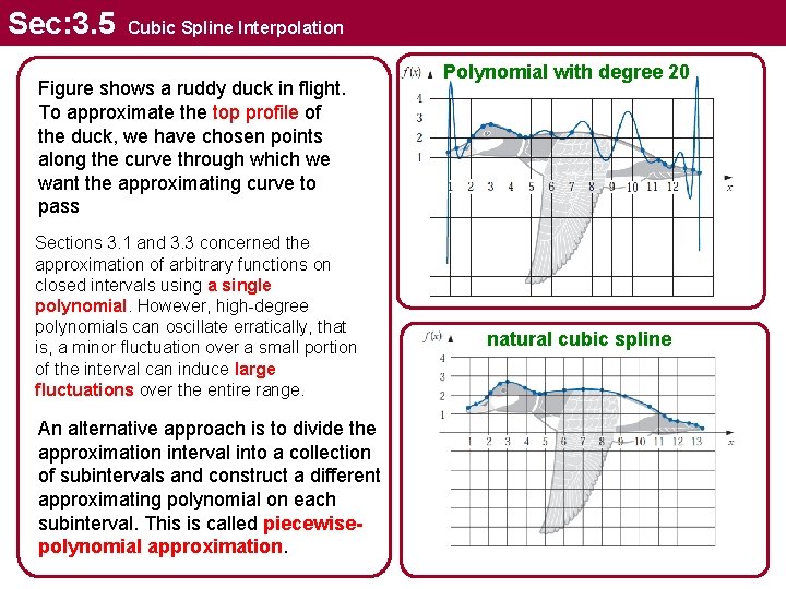
Sec: 3. 5 Cubic Spline Interpolation Figure shows a ruddy duck in flight. To approximate the top profile of the duck, we have chosen points along the curve through which we want the approximating curve to pass Sections 3. 1 and 3. 3 concerned the approximation of arbitrary functions on closed intervals using a single polynomial. However, high-degree polynomials can oscillate erratically, that is, a minor fluctuation over a small portion of the interval can induce large fluctuations over the entire range. An alternative approach is to divide the approximation interval into a collection of subintervals and construct a different approximating polynomial on each subinterval. This is called piecewisepolynomial approximation. Polynomial with degree 20 natural cubic spline
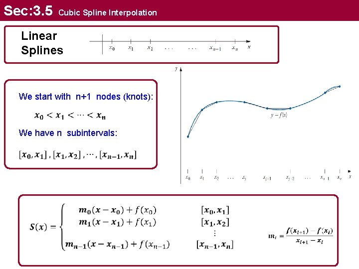
Sec: 3. 5 Cubic Spline Interpolation Linear Splines We start with n+1 nodes (knots): We have n subintervals:
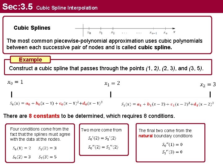
Sec: 3. 5 Cubic Spline Interpolation Cubic Splines The most common piecewise-polynomial approximation uses cubic polynomials between each successive pair of nodes and is called cubic spline. Example Construct a cubic spline that passes through the points (1, 2), (2, 3), and (3, 5). There are 8 constants to be determined, which requires 8 conditions. Four conditions come from the fact that the splines must agree with the data at the nodes. Two more come from The final two come from the natural boundary conditions
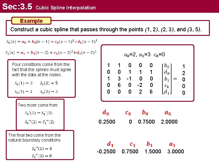
Sec: 3. 5 Cubic Spline Interpolation Example Construct a cubic spline that passes through the points (1, 2), (2, 3), and (3, 5). Four conditions come from the fact that the splines must agree with the data at the nodes. 1 0 0 1 0 3 6 0 0 1 -1 0 0 0 1 0 -2 2 0 1 0 0 6 1 2 0 0 0 Two more come from 0. 2500 0 0. 7500 -0. 2500 0. 7500 2. 0000 The final two come from the natural boundary conditions 1. 5000 3. 0000
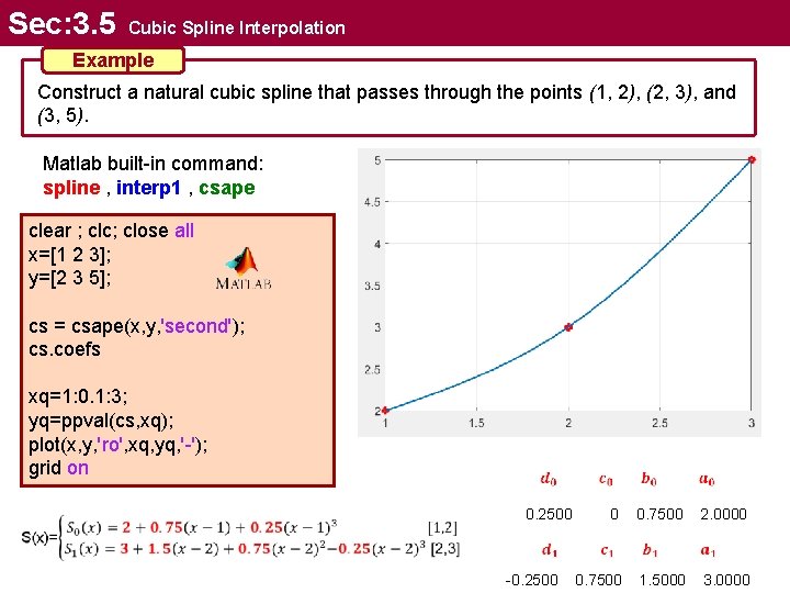
Sec: 3. 5 Cubic Spline Interpolation Example Construct a natural cubic spline that passes through the points (1, 2), (2, 3), and (3, 5). Matlab built-in command: spline , interp 1 , csape clear ; clc; close all x=[1 2 3]; y=[2 3 5]; cs = csape(x, y, 'second'); cs. coefs xq=1: 0. 1: 3; yq=ppval(cs, xq); plot(x, y, 'ro', xq, yq, '-'); grid on 0. 2500 -0. 2500 0 0. 7500 2. 0000 0. 7500 1. 5000 3. 0000
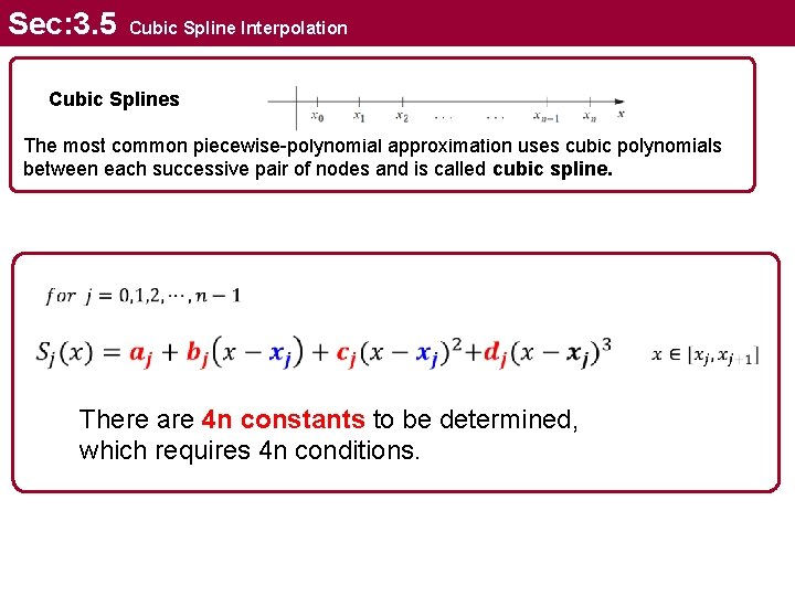
Sec: 3. 5 Cubic Spline Interpolation Cubic Splines The most common piecewise-polynomial approximation uses cubic polynomials between each successive pair of nodes and is called cubic spline. There are 4 n constants to be determined, which requires 4 n conditions.
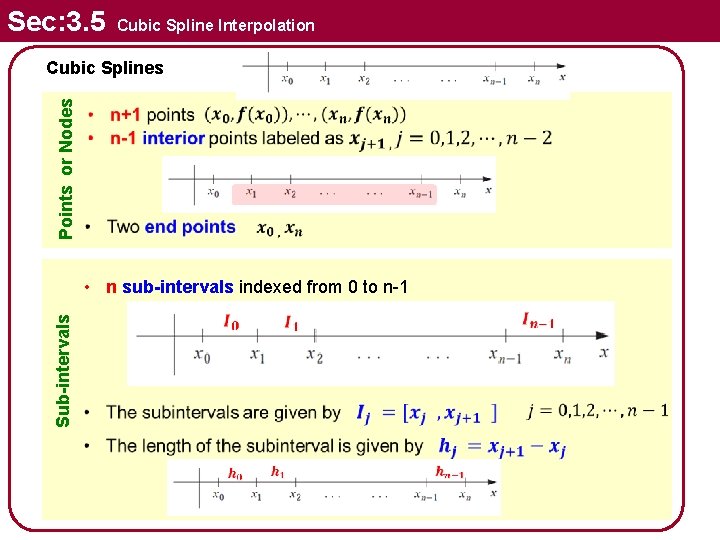
Sec: 3. 5 Cubic Spline Interpolation Points or Nodes Cubic Splines Sub-intervals • n sub-intervals indexed from 0 to n-1
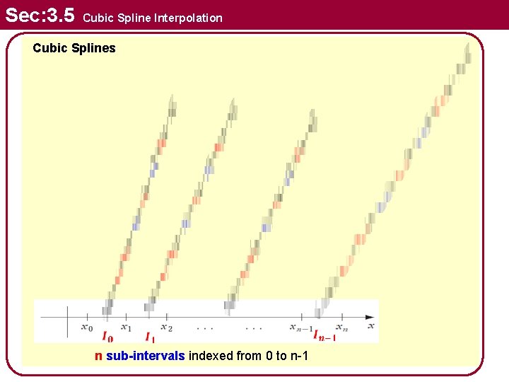
Sec: 3. 5 Cubic Spline Interpolation Cubic Splines n sub-intervals indexed from 0 to n-1
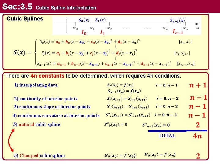
Sec: 3. 5 Cubic Spline Interpolation Cubic Splines There are 4 n constants to be determined, which requires 4 n conditions. 1) interpolating data 2) continuity at interior points 3) continuous slope at interior points 4) continuous curvature at interior points 5) natural cubic spline TOTAL 5) Clamped cubic spline
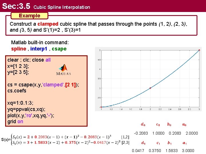
Sec: 3. 5 Cubic Spline Interpolation Example Construct a clamped cubic spline that passes through the points (1, 2), (2, 3), and (3, 5) and S’(1)=2 , S’(3)=1 Matlab built-in command: spline , interp 1 , csape clear ; clc; close all x=[1 2 3]; y=[2 3 5]; cs = csape(x, y, ‘clamped‘, [2 1]); cs. coefs xq=1: 0. 1: 3; yq=ppval(cs, xq); plot(x, y, 'ro', xq, yq, '-'); grid on -0. 2083 0. 0417 1. 0000 0. 3750 0. 2083 1. 5833 2. 0000 3. 0000
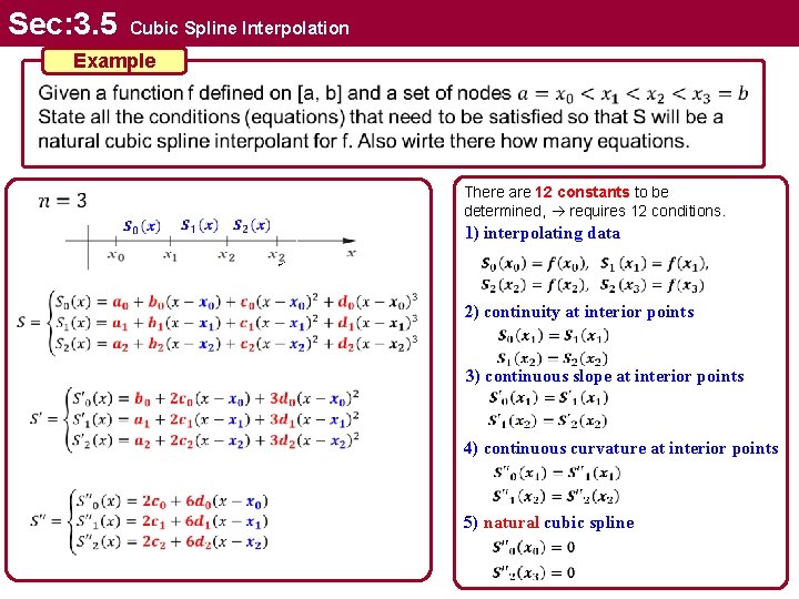
Sec: 3. 5 Cubic Spline Interpolation Example There are 12 constants to be determined, requires 12 conditions. 1) interpolating data 2) continuity at interior points 3) continuous slope at interior points 4) continuous curvature at interior points 5) natural cubic spline
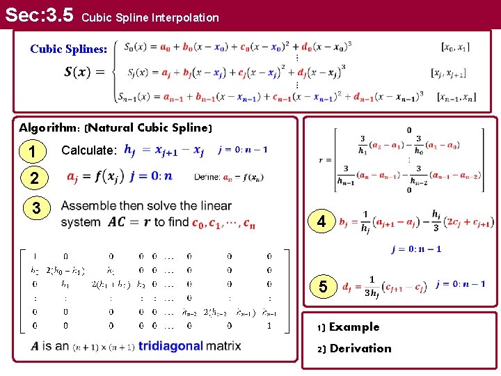
Sec: 3. 5 Cubic Spline Interpolation Cubic Splines: Algorithm: (Natural Cubic Spline) 1 Calculate: 2 3 4 5 1) Example 2) Derivation
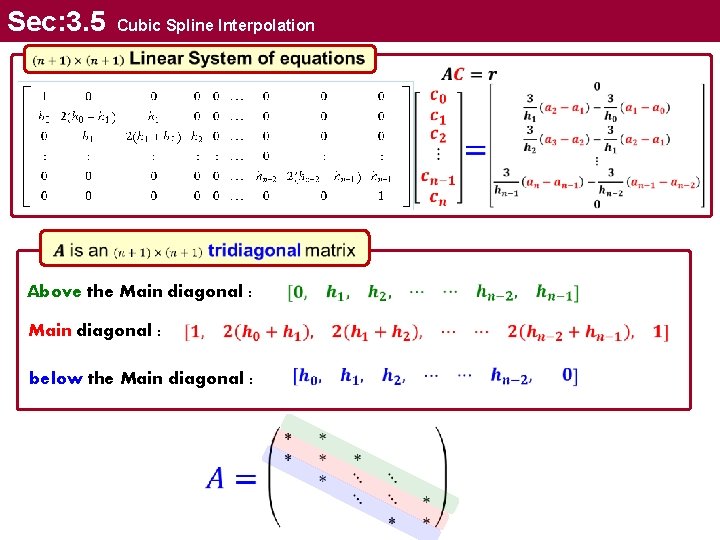
Sec: 3. 5 Cubic Spline Interpolation Above the Main diagonal : below the Main diagonal :
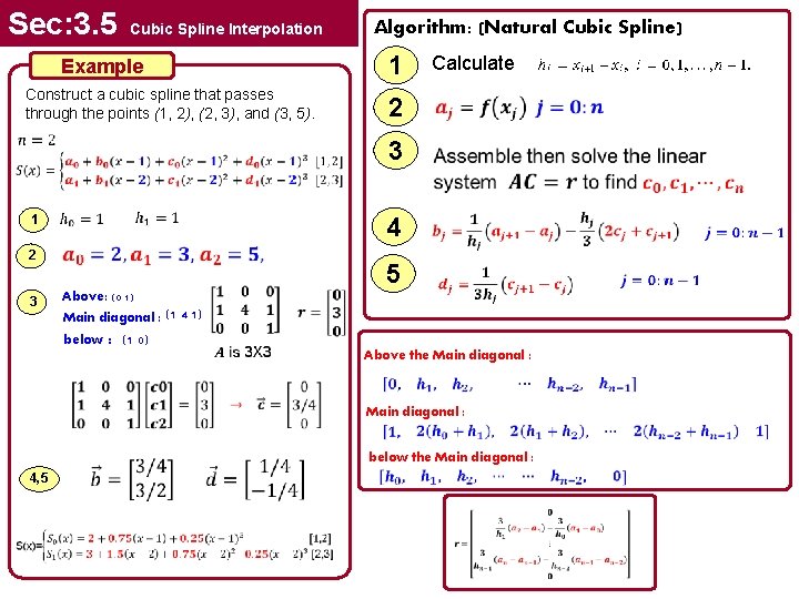
Sec: 3. 5 Cubic Spline Interpolation Example Construct a cubic spline that passes through the points (1, 2), (2, 3), and (3, 5). Algorithm: (Natural Cubic Spline) 1 Calculate: 2 3 1 4 2 3 5 Above: (0 1) Main diagonal : (1 4 1) below : (1 0) Above the Main diagonal : below the Main diagonal : 4, 5
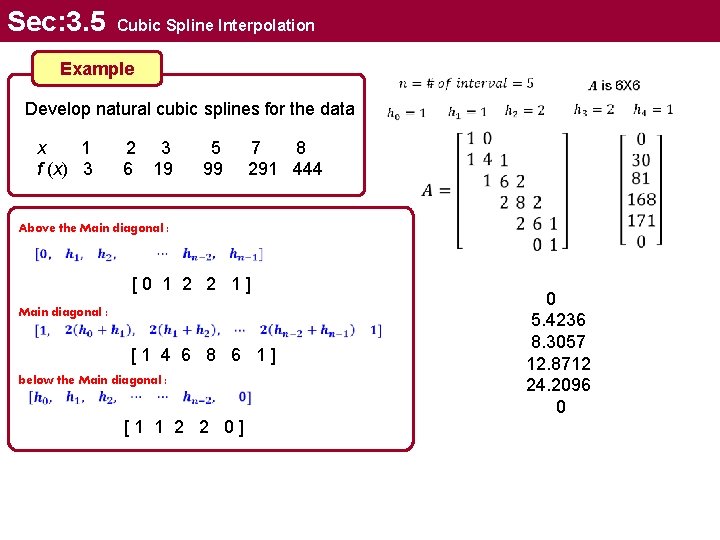
Sec: 3. 5 Cubic Spline Interpolation Example Develop natural cubic splines for the data x 1 f (x) 3 2 3 6 19 5 99 7 8 291 444 Above the Main diagonal : [0 1 2 2 1] Main diagonal : [1 4 6 8 6 1] below the Main diagonal : [1 1 2 2 0] 0 5. 4236 8. 3057 12. 8712 24. 2096 0
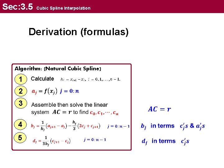
Sec: 3. 5 Cubic Spline Interpolation Derivation (formulas) Algorithm: (Natural Cubic Spline) 1 2 3 4 5 Calculate:
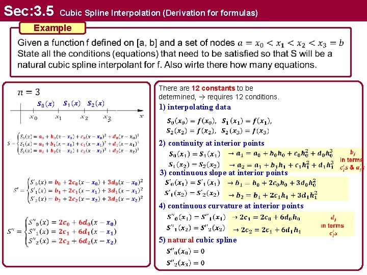
Sec: 3. 5 Cubic Spline Interpolation (Derivation formulas) Example There are 12 constants to be determined, requires 12 conditions. 1) interpolating data 2) continuity at interior points 3) continuous slope at interior points 4) continuous curvature at interior points 5) natural cubic spline
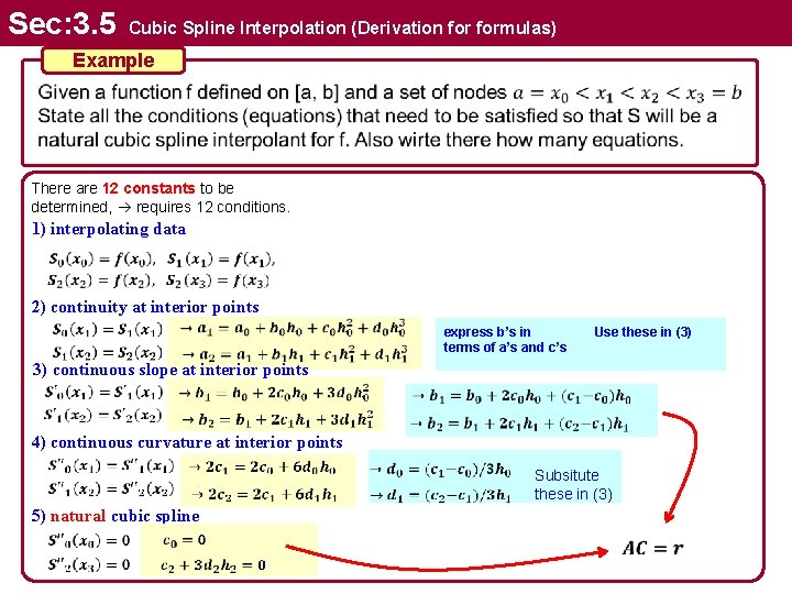
Sec: 3. 5 Cubic Spline Interpolation (Derivation formulas) Example There are 12 constants to be determined, requires 12 conditions. 1) interpolating data 2) continuity at interior points express b’s in terms of a’s and c’s Use these in (3) 3) continuous slope at interior points 4) continuous curvature at interior points Subsitute these in (3) 5) natural cubic spline
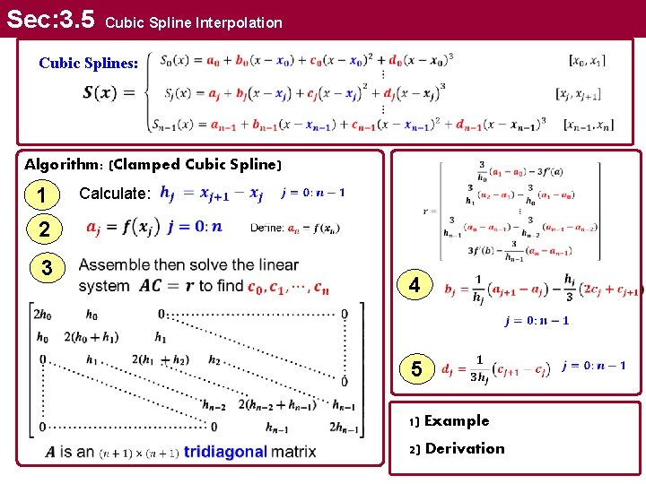
Sec: 3. 5 Cubic Spline Interpolation Cubic Splines: Algorithm: (Clamped Cubic Spline) 1 Calculate: 2 3 4 5 1) Example 2) Derivation
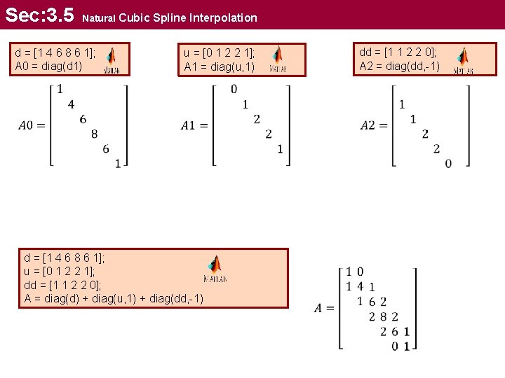
Sec: 3. 5 Natural Cubic Spline Interpolation d = [1 4 6 8 6 1]; A 0 = diag(d 1) u = [0 1 2 2 1]; A 1 = diag(u, 1) d = [1 4 6 8 6 1]; u = [0 1 2 2 1]; dd = [1 1 2 2 0]; A = diag(d) + diag(u, 1) + diag(dd, -1) dd = [1 1 2 2 0]; A 2 = diag(dd, -1)
![Sec: 3. 5 Cubic Spline Interpolation function [a, b, c, d, coeff] = myspline(x, Sec: 3. 5 Cubic Spline Interpolation function [a, b, c, d, coeff] = myspline(x,](http://slidetodoc.com/presentation_image_h2/3f9bb31ebb2a64b465b6206980bf4a4e/image-22.jpg)
Sec: 3. 5 Cubic Spline Interpolation function [a, b, c, d, coeff] = myspline(x, y) n 1=length(y); n = n 1 -1; for i=1: n; h(i) = x(i+1)-x(i); end v=zeros(n+1, 1); for i=2: n v(i) = 3*( (y(i+1)-y(i))/h(i) - (y(i)-y(i-1))/h(i-1) ); end md(1) = 1; ud(1)=0; for i=2: n md(i) = 2*(h(i-1)+h(i)); ud(i) = h(i); end md = [md , 1]; for i=1: n-1 dd(i) = h(i); end dd = [ dd 0]; A = zeros(n+1, n+1); A = diag(md) + diag(ud, 1) + diag(dd, -1); c = Av; for i=1: n+1; a(i) = y(i); end for i=1: n d(i) = ( c(i+1) - c(i) )/(3*h(i)); b(i) = (a(i+1)-a(i))/h(i) - h(i)*( 2*c(i) + c(i+1))/3; end coeff =[d' c(1: n) b' a(1: n)']; end Above the Main diagonal : below the Main diagonal : Here we calculate spline coefficients using myspline. m and store them in coeff matrix. Also we use MATLAB built-in command ‘csape’ to calculate the coefficients and store them in cof. clear, clc x=[1 2 3 5 7 8]; y=[3 6 19 99 291 444]; [a, b, c, d, coeff] = myspline(x, y); cs = csape(x, y, 'second'); cof=cs. coefs coeff
Sec: 3. 5 Cubic Spline Interpolation 1) Parametric Curves 2) MULTIDIMENSIONAL INTERPOLATION
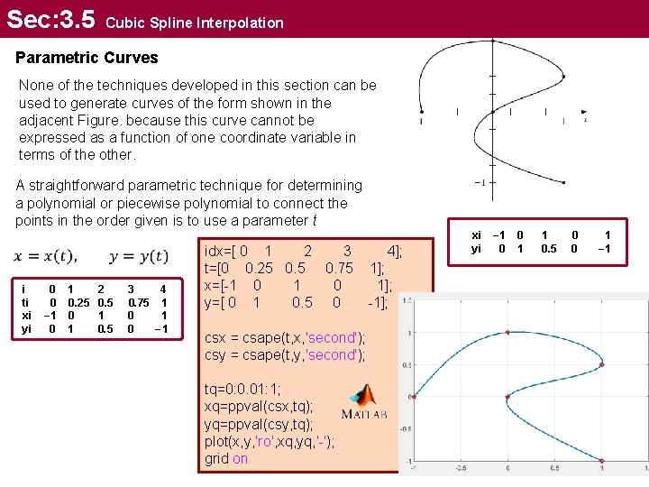
Sec: 3. 5 Cubic Spline Interpolation Parametric Curves None of the techniques developed in this section can be used to generate curves of the form shown in the adjacent Figure. because this curve cannot be expressed as a function of one coordinate variable in terms of the other. A straightforward parametric technique for determining a polynomial or piecewise polynomial to connect the points in the order given is to use a parameter t i ti xi yi 0 0 − 1 0. 25 0 1 2 0. 5 1 0. 5 3 4 0. 75 1 0 − 1 idx=[ 0 1 2 3 t=[0 0. 25 0. 75 x=[-1 0 y=[ 0 1 0. 5 0 csx = csape(t, x, 'second'); csy = csape(t, y, 'second'); tq=0: 0. 01: 1; xq=ppval(csx, tq); yq=ppval(csy, tq); plot(x, y, 'ro', xq, yq, '-'); grid on 4]; 1]; -1]; xi yi − 1 0 0 1 1 0. 5 0 0 1 − 1
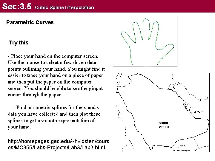
Sec: 3. 5 Cubic Spline Interpolation Parametric Curves Try this - Place your hand on the computer screen. Use the mouse to select a few dozen data points outlining your hand. You might find it easier to trace your hand on a piece of paper and then put the paper on the computer screen. You should be able to see the ginput cursor through the paper. - Find parametric splines for the x and y data you have collected and then plot these splines to get a smooth representation of your hand. http: //homepages. gac. edu/~hvidsten/cours es/MC 355/Labs-Projects/Lab 3. html
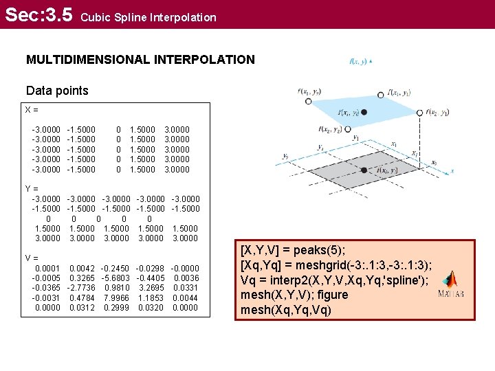
Sec: 3. 5 Cubic Spline Interpolation MULTIDIMENSIONAL INTERPOLATION Data points X= -3. 0000 -1. 5000 0 0 1. 5000 3. 0000 Y= -3. 0000 -1. 5000 0 0 0 1. 5000 3. 0000 -3. 0000 -1. 5000 3. 0000 V= 0. 0001 0. 0042 -0. 2450 -0. 0298 -0. 0000 -0. 0005 0. 3265 -5. 6803 -0. 4405 0. 0036 -0. 0365 -2. 7736 0. 9810 3. 2695 0. 0331 -0. 0031 0. 4784 7. 9966 1. 1853 0. 0044 0. 0000 0. 0312 0. 2999 0. 0320 0. 0000 [X, Y, V] = peaks(5); [Xq, Yq] = meshgrid(-3: . 1: 3, -3: . 1: 3); Vq = interp 2(X, Y, V, Xq, Yq, 'spline'); mesh(X, Y, V); figure mesh(Xq, Yq, Vq)
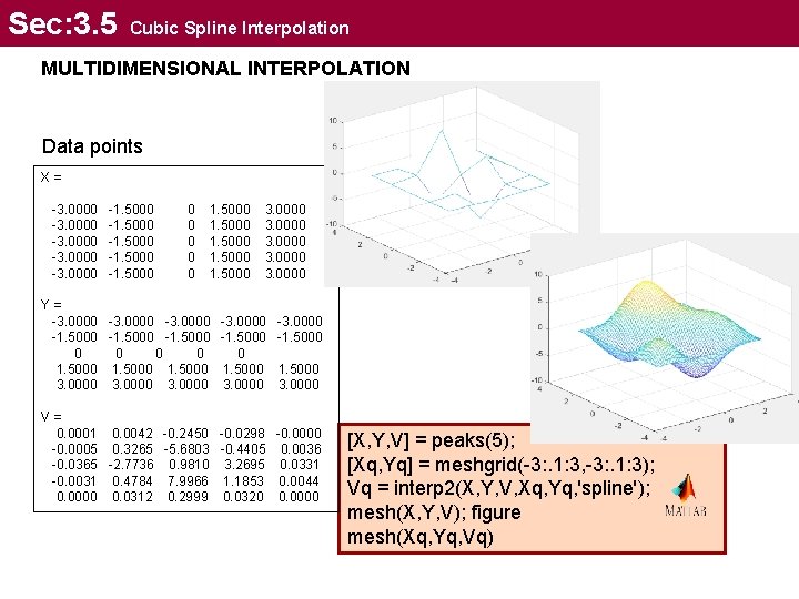
Sec: 3. 5 Cubic Spline Interpolation MULTIDIMENSIONAL INTERPOLATION Data points X= -3. 0000 -1. 5000 0 0 1. 5000 3. 0000 Y= -3. 0000 -1. 5000 0 0 0 1. 5000 3. 0000 -3. 0000 -1. 5000 3. 0000 V= 0. 0001 0. 0042 -0. 2450 -0. 0298 -0. 0000 -0. 0005 0. 3265 -5. 6803 -0. 4405 0. 0036 -0. 0365 -2. 7736 0. 9810 3. 2695 0. 0331 -0. 0031 0. 4784 7. 9966 1. 1853 0. 0044 0. 0000 0. 0312 0. 2999 0. 0320 0. 0000 [X, Y, V] = peaks(5); [Xq, Yq] = meshgrid(-3: . 1: 3, -3: . 1: 3); Vq = interp 2(X, Y, V, Xq, Yq, 'spline'); mesh(X, Y, V); figure mesh(Xq, Yq, Vq)
- Slides: 27