Searching for with CMS Sezen Sekmen CERN IPMLHC

Searching for with CMS Sezen Sekmen, CERN IPMLHC 2013, 7 -11 Sept 2013 IPM, Tehran 1

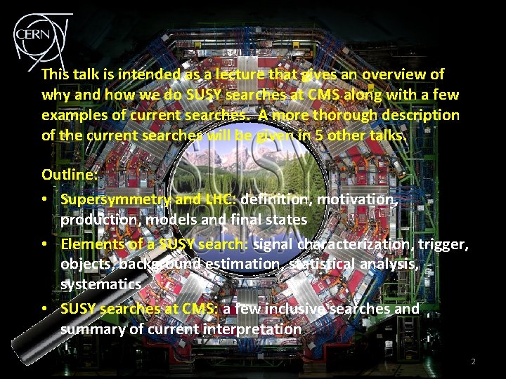
This talk is intended as a lecture that gives an overview of why and how we do SUSY searches at CMS along with a few examples of current searches. A more thorough description of the current searches will be given in 5 other talks. Outline: • Supersymmetry and LHC: definition, motivation, production, models and final states • Elements of a SUSY search: signal characterization, trigger, objects, background estimation, statistical analysis, systematics • SUSY searches at CMS: a few inclusive searches and summary of current interpretation 2

SUSY and the LHC 3

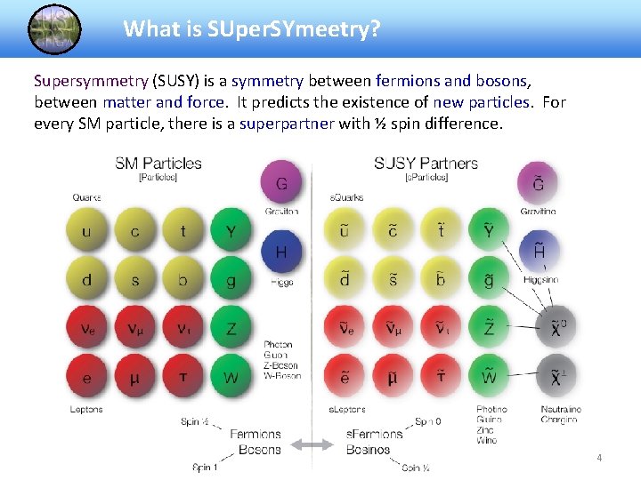
What is SUper. SYmeetry? Supersymmetry (SUSY) is a symmetry between fermions and bosons, between matter and force. It predicts the existence of new particles. For every SM particle, there is a superpartner with ½ spin difference. 4

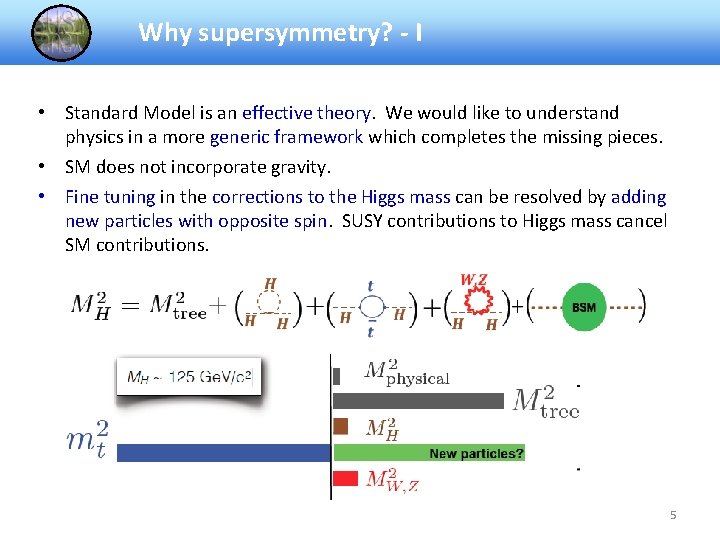
Why supersymmetry? - I • Standard Model is an effective theory. We would like to understand physics in a more generic framework which completes the missing pieces. • SM does not incorporate gravity. • Fine tuning in the corrections to the Higgs mass can be resolved by adding new particles with opposite spin. SUSY contributions to Higgs mass cancel SM contributions. 5

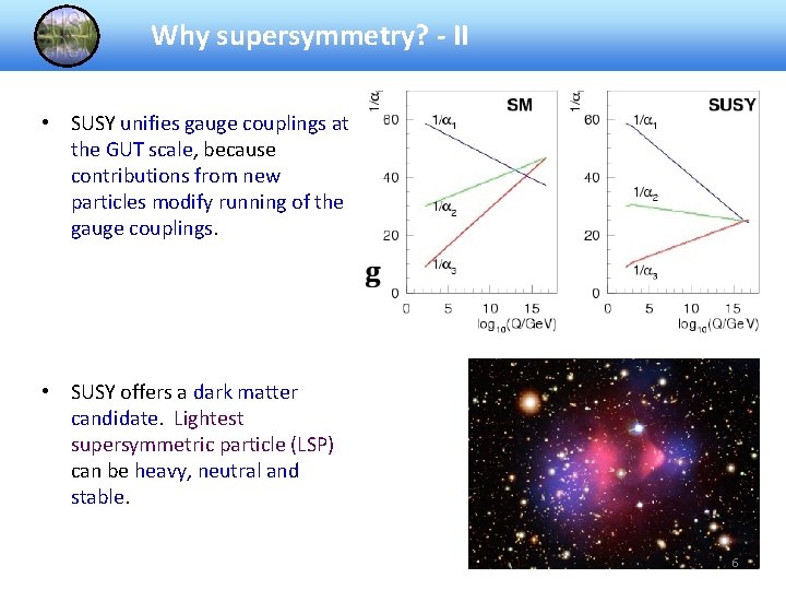
Why supersymmetry? - II • SUSY unifies gauge couplings at the GUT scale, because contributions from new particles modify running of the gauge couplings. • SUSY offers a dark matter candidate. Lightest supersymmetric particle (LSP) can be heavy, neutral and stable. 6

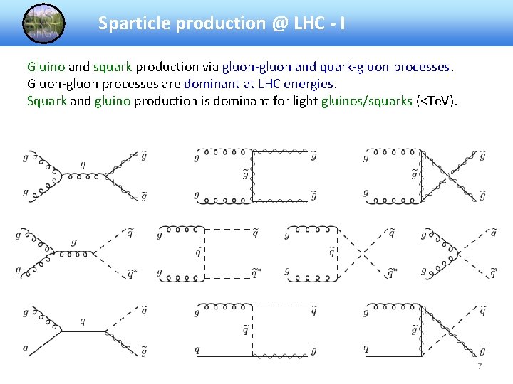
Sparticle production @ LHC - I Gluino and squark production via gluon-gluon and quark-gluon processes. Gluon-gluon processes are dominant at LHC energies. Squark and gluino production is dominant for light gluinos/squarks (<Te. V). 7

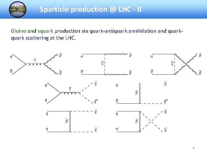
Sparticle production @ LHC - II Gluino and squark production via quark-antiquark annihilation and quark scattering at the LHC. 8

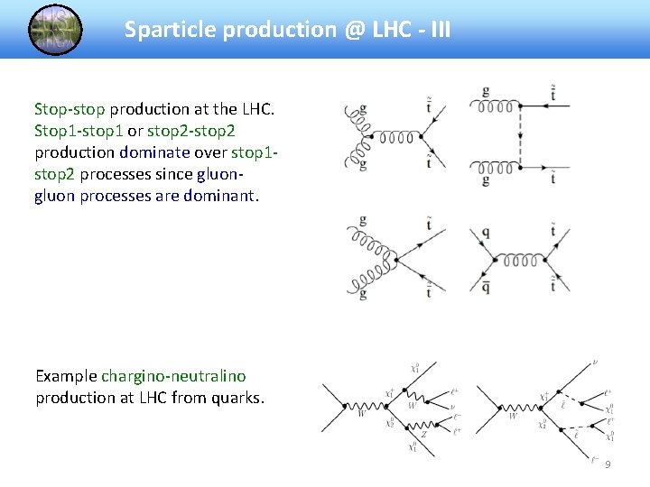
Sparticle production @ LHC - III Stop-stop production at the LHC. Stop 1 -stop 1 or stop 2 -stop 2 production dominate over stop 1 stop 2 processes since gluon processes are dominant. Example chargino-neutralino production at LHC from quarks. 9

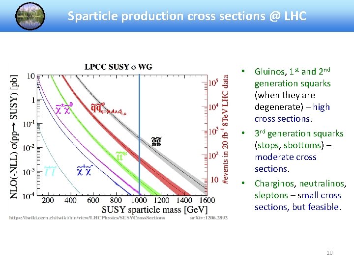
Sparticle production cross sections @ LHC • Gluinos, 1 st and 2 nd generation squarks (when they are degenerate) – high cross sections. • 3 rd generation squarks (stops, sbottoms) – moderate cross sections. • Charginos, neutralinos, sleptons – small cross sections, but feasible. 10

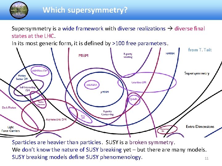
Which supersymmetry? Supersymmetry is a wide framework with diverse realizations diverse final states at the LHC. In its most generic form, it is defined by >100 free parameters. from T. Tait Sparticles are heavier than particles. SUSY is a broken symmetry. We don’t know the nature of SUSY breaking yet – but there are many models. SUSY breaking models define SUSY phenomenology. 11

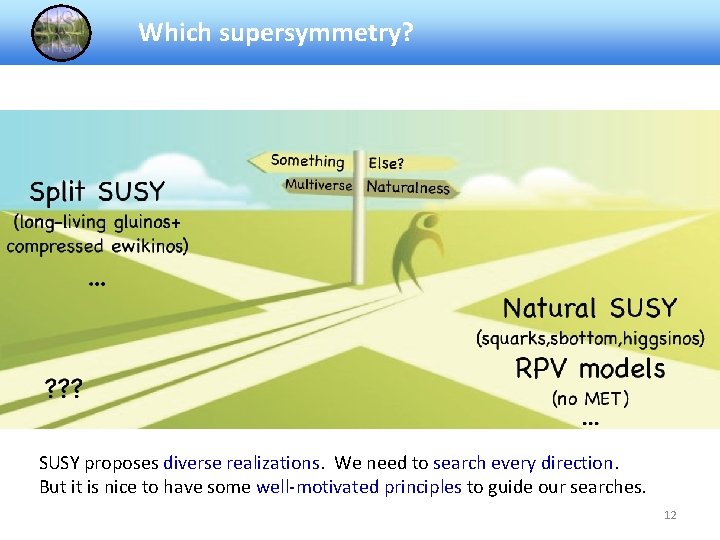
Which supersymmetry? SUSY proposes diverse realizations. We need to search every direction. But it is nice to have some well-motivated principles to guide our searches. 12

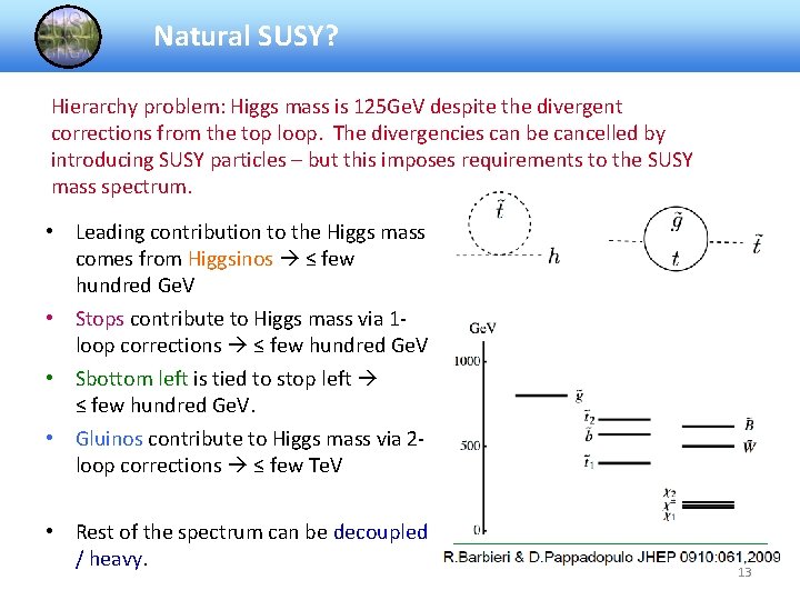
Natural SUSY? Hierarchy problem: Higgs mass is 125 Ge. V despite the divergent corrections from the top loop. The divergencies can be cancelled by introducing SUSY particles – but this imposes requirements to the SUSY mass spectrum. • Leading contribution to the Higgs mass comes from Higgsinos ≤ few hundred Ge. V • Stops contribute to Higgs mass via 1 loop corrections ≤ few hundred Ge. V • Sbottom left is tied to stop left ≤ few hundred Ge. V. • Gluinos contribute to Higgs mass via 2 loop corrections ≤ few Te. V • Rest of the spectrum can be decoupled / heavy. 13

A generic framework: p. MSSM Given that we are not convinced by a theorietical motivation, we can consider a more generic framework. • p(henomenological)MSSM is a 19 -dimensional parameterization of MSSM at the SUSY scale. • p. MSSM is defined by • 3 gaugino mass parameters • 10 sfermion mass parameters • 3 trilinear couplings • ratio of Higgs VEVs tanβ, Higgsino mass parameter μ and pseudoscalar Higgs mass m. A • plus a set of minimal assumptions. • It is a full model with no assumptions on the nature of SUSY breaking mechanism and no correlations between the sparticle masses. It allows to make generic statements on sparticle masses. 14

Simplified models Or maybe we would like to simply have a way of modeling SUSY-like final states one-by-one in terms of an effective framework? • A simplified model is defined by a set of hypothetical particles and a sequence of their production and decays. • For each simplified model, values for the product of the experimental acceptance and efficiency (A X e) are calculated to translate a number of signal events into a signal cross section. • From this information, a 95% confidence level upper limit on the product of the cross section and branching fraction is derived as a function of the particle mass. • Only the production process of two particles is considered. • Each particle decays directly or via a cascade to particles X + a neutral, undetected particle (i. e. , the LSP. ) 15

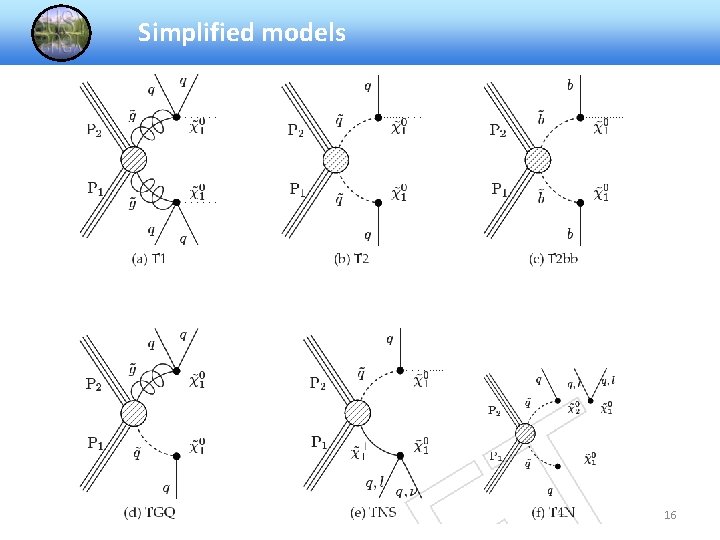
Simplified models 16

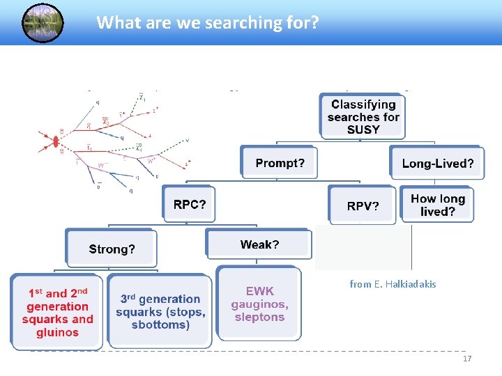
What are we searching for? from E. Halkiadakis 17

Elements of a SUSY search 18

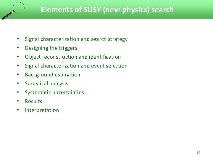
Elements of SUSY (new physics) search • • • Signal characterization and search strategy Designing the triggers Object reconstruction and identification Signal characterization and event selection Background estimation Statistical analysis Systematic uncertainties Results Interpretation 19

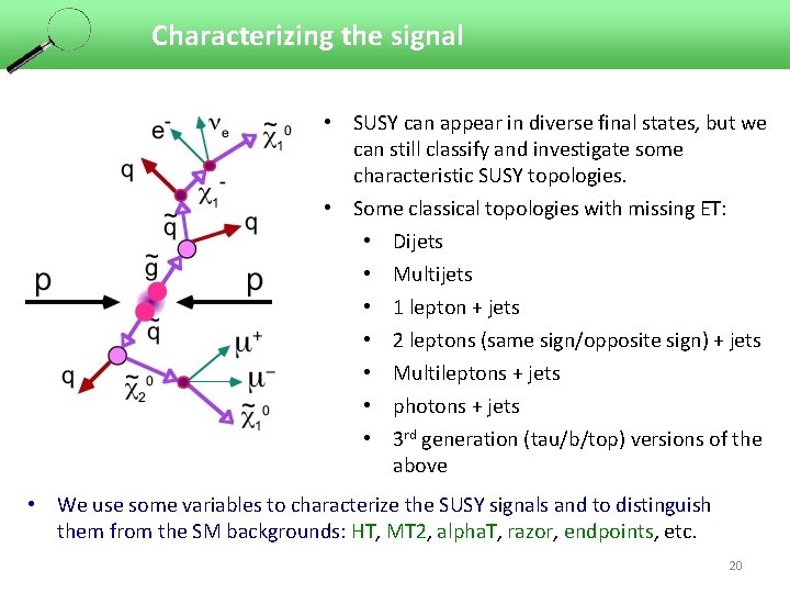
Characterizing the signal • SUSY can appear in diverse final states, but we ü Defined can still classify and investigate some by an effective characteristic SUSY topologies. Lagrangian • Some classical topologies with missing ET: • Dijets • Multijets • 1 lepton + jets • 2 leptons (same sign/opposite sign) + jets • Multileptons + jets • photons + jets • 3 rd generation (tau/b/top) versions of the above • We use some variables to characterize the SUSY signals and to distinguish them from the SM backgrounds: HT, MT 2, alpha. T, razor, endpoints, etc. 20

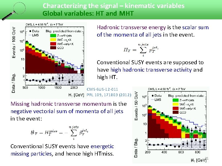
Characterizing the signal – kinematic variables Global variables: HT and MHT Hadronic transverse energy is the scalar sum of the momenta of all jets in the event. ü Defined by an effective Lagrangian Conventional SUSY events are supposed to have high hadronic transverse activity and high HT. CMS-SUS-12 -011 PRL 109, 171803 (2012) Missing hadronic transverse momentum is the negative vectorial sum of momenta of all jets in the event: Conventional SUSY events have energetic missing particles, and hence high HTmiss. 21

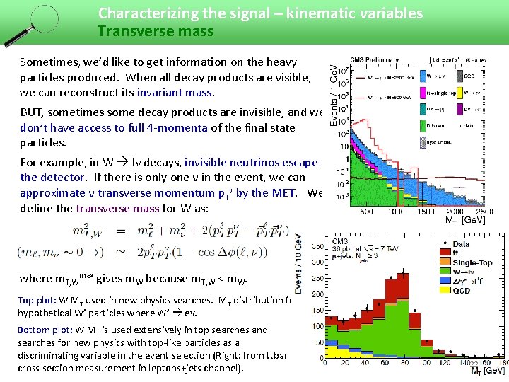
Characterizing the signal – kinematic variables Transverse mass Sometimes, we’d like to get information on the heavy particles produced. When all decay products are visible, we can reconstruct its invariant mass. BUT, sometimes some decay products are invisible, and we don’t have access to full 4 -momenta of the final state particles. For example, in W lν decays, invisible neutrinos escape the detector. If there is only one ν in the event, we can approximate ν transverse momentum p. Tν by the MET. We define the transverse mass for W as: where m. T, Wmax gives m. W because m. T, W < m. W. Top plot: W MT used in new physics searches. MT distribution for hypothetical W’ particles where W’ ev. Bottom plot: W MT is used extensively in top searches and searches for new physics with top-like particles as a discriminating variable in the event selection (Right: from ttbar cross section measurement in leptons+jets channel). 22

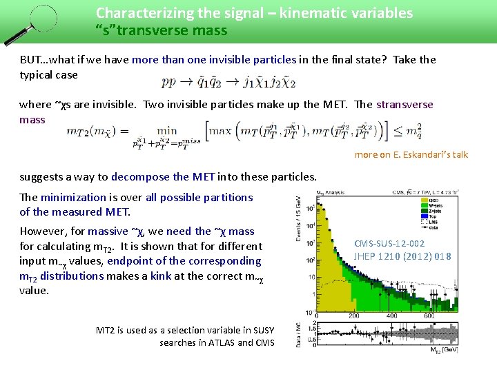
Characterizing the signal – kinematic variables “s”transverse mass BUT…what if we have more than one invisible particles in the final state? Take the typical case where ~χs are invisible. Two invisible particles make up the MET. The stransverse mass more on E. Eskandari’s talk suggests a way to decompose the MET into these particles. The minimization is over all possible partitions of the measured MET. However, for massive ~χ, we need the ~χ mass for calculating m. T 2. It is shown that for different input m~χ values, endpoint of the corresponding m. T 2 distributions makes a kink at the correct m~χ value. CMS-SUS-12 -002 JHEP 1210 (2012) 018 MT 2 is used as a selection variable in SUSY searches in ATLAS and CMS 23

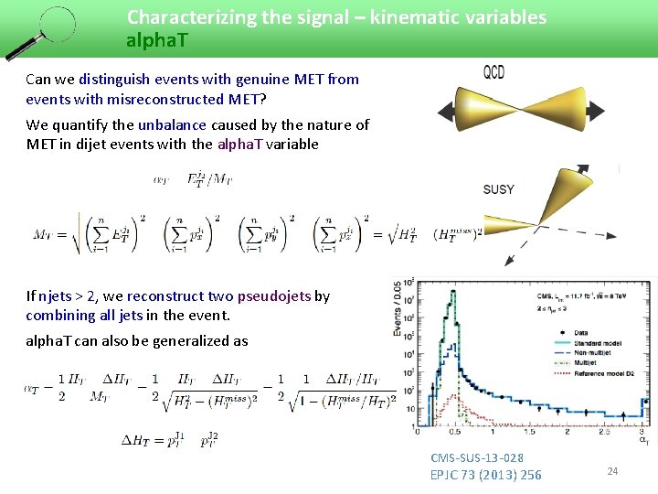
Characterizing the signal – kinematic variables alpha. T Can we distinguish events with genuine MET from events with misreconstructed MET? We quantify the unbalance caused by the nature of MET in dijet events with the alpha. T variable If njets > 2, we reconstruct two pseudojets by combining all jets in the event. alpha. T can also be generalized as CMS-SUS-13 -028 EPJC 73 (2013) 256 24

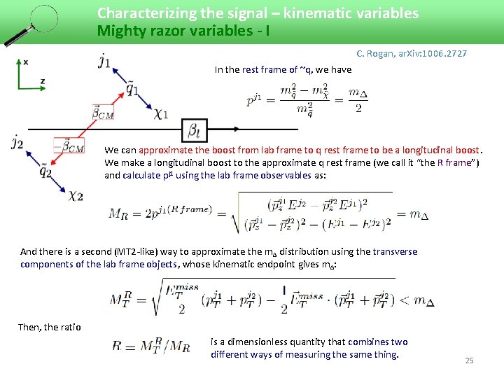
Characterizing the signal – kinematic variables Mighty razor variables - I C. Rogan, ar. Xiv: 1006. 2727 In the rest frame of ~q, we have We can approximate the boost from lab frame to q rest frame to be a longitudinal boost. We make a longitudinal boost to the approximate q rest frame (we call it “the R frame”) and calculate pj 1 using the lab frame observables as: And there is a second (MT 2 -like) way to approximate the mΔ distribution using the transverse components of the lab frame objects, whose kinematic endpoint gives mΔ: Then, the ratio is a dimensionless quantity that combines two different ways of measuring the same thing. 25

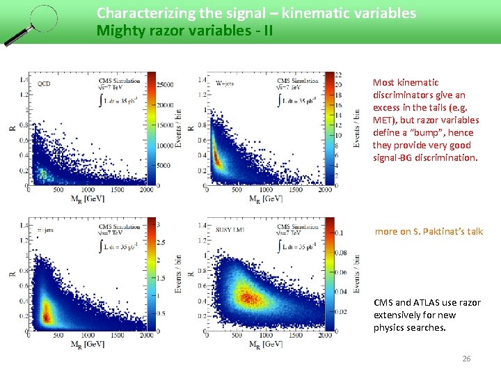
Characterizing the signal – kinematic variables Mighty razor variables - II Most kinematic discriminators give an excess in the tails (e. g. MET), but razor variables define a “bump”, hence they provide very good signal-BG discrimination. more on S. Paktinat’s talk CMS and ATLAS use razor extensively for new physics searches. 26

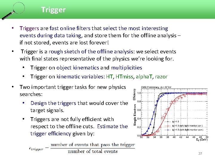
Trigger • Triggers are fast online filters that select the most interesting events during data taking, and store them for the offline analysis – if not stored, events are lost forever! • Trigger is a rough sketch of the offline analysis: we select events with final states representative of the physics we’re looking for. • Trigger on object kinematics and multiplicities • Trigger on kinematic variables: HT, HTmiss, alpha. T, razor • Two important trigger tasks for new physics searches: • Design the triggers that would cover the target signals. • Triggers are not fully efficient with respect to the offline cuts. Estimate the trigger efficiency given by: 27

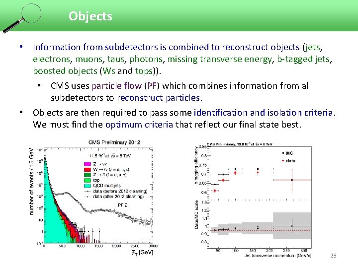
Objects • Information from subdetectors is combined to reconstruct objects (jets, electrons, muons, taus, photons, missing transverse energy, b-tagged jets, boosted objects (Ws and tops)). • CMS uses particle flow (PF) which combines information from all subdetectors to reconstruct particles. • Objects are then required to pass some identification and isolation criteria. We must find the optimum criteria that reflect our final state best. 28

Event selection: principles • Characterize the signal. Find final state topologies and kinematic variables that discriminate the signal from the backgrounds. Multijets? Oppositesign dileptons? b-rich? Discriminating kinematic properties? • Look for statistically significant signal regions. There should be sufficient number of events, and sufficient number of predicted signal events over the expected background. • Make sure that there is a way to estimate the expected background in the signal region. • Make sure that the offline selection corresponds to a region where the trigger efficiency is well-modeled. • Make sure that the selection variables are reconstructed and identified in well-defined regions of the detector (not feasible to design a search with forward electrons). • Numerous multivariate methods exist for selection optimization: rectangular cuts, fisher discrimination, likelihoods, neural networks, decision trees, support vector machines, … 29

BAAACKGROOOOUNDSSS!!! 30

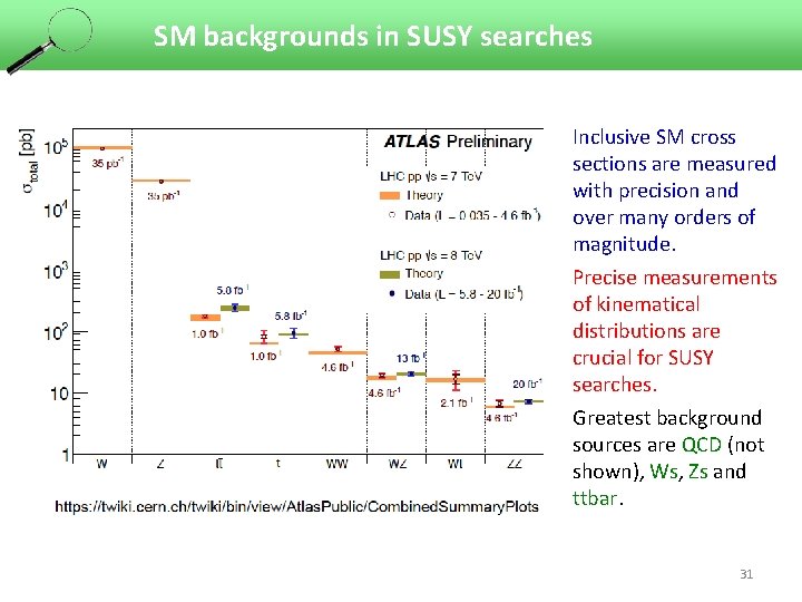
SM backgrounds in SUSY searches Inclusive SM cross sections are measured with precision and over many orders of magnitude. Precise measurements of kinematical distributions are crucial for SUSY searches. Greatest background sources are QCD (not shown), Ws, Zs and ttbar. 31

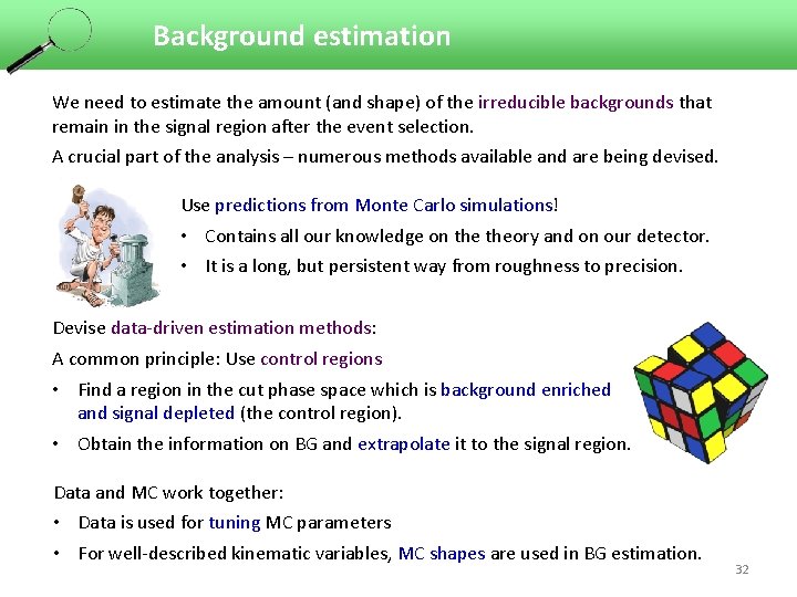
Background estimation We need to estimate the amount (and shape) of the irreducible backgrounds that remain in the signal region after the event selection. A crucial part of the analysis – numerous methods available and are being devised. Use predictions from Monte Carlo simulations! • Contains all our knowledge on theory and on our detector. • It is a long, but persistent way from roughness to precision. Devise data-driven estimation methods: A common principle: Use control regions • Find a region in the cut phase space which is background enriched and signal depleted (the control region). • Obtain the information on BG and extrapolate it to the signal region. Data and MC work together: • Data is used for tuning MC parameters • For well-described kinematic variables, MC shapes are used in BG estimation. 32

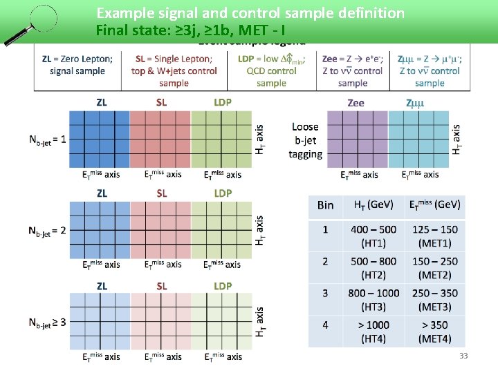
Example signal and control sample definition Final state: ≥ 3 j, ≥ 1 b, MET - I 33

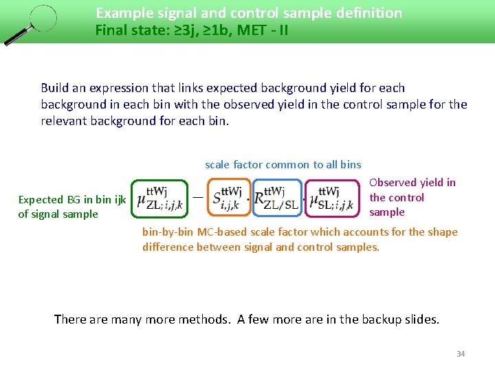
Example signal and control sample definition Final state: ≥ 3 j, ≥ 1 b, MET - II Build an expression that links expected background yield for each background in each bin with the observed yield in the control sample for the relevant background for each bin. scale factor common to all bins Expected BG in bin ijk of signal sample Observed yield in the control sample bin-by-bin MC-based scale factor which accounts for the shape difference between signal and control samples. There are many more methods. A few more are in the backup slides. 34

Statistical modeling and likelihood analysis • The statistical model of an analysis provides the complete mathematical description of that analysis. • It relates the observed quantities x to the parameters θ through the probability density p(x|θ). • The likelihood L(θ) = p(X 0|θ) is the probability density p(x|θ) evaluated at the observed values X 0 of the observables x. • A likelihood is the starting point of any serious interpretation. 35

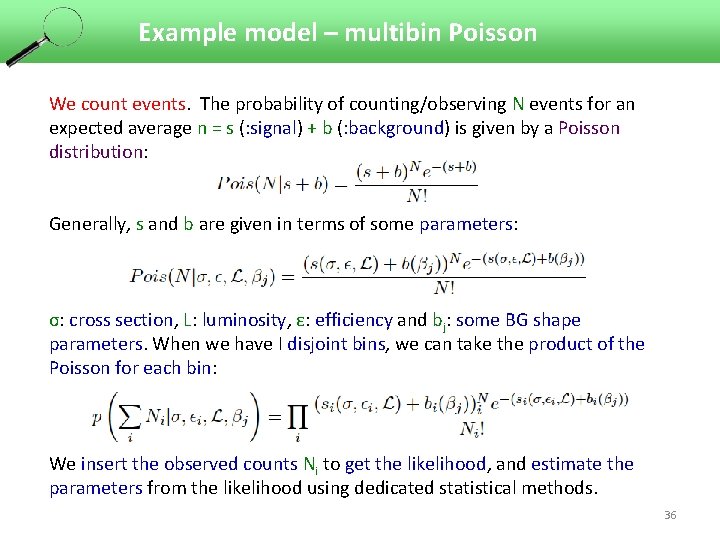
Example model – multibin Poisson We count events. The probability of counting/observing N events for an expected average n = s (: signal) + b (: background) is given by a Poisson distribution: Generally, s and b are given in terms of some parameters: σ: cross section, L: luminosity, ε: efficiency and bj: some BG shape parameters. When we have I disjoint bins, we can take the product of the Poisson for each bin: We insert the observed counts Ni to get the likelihood, and estimate the parameters from the likelihood using dedicated statistical methods. 36

Results and interpretation • An experimental result is the empirical outcome of the experiment, such as an event count, or the measurement of some physical quantity, such as mass, cross section, spin, charge asymmetry, kinematic edges, etc. • Given an experimental result, we can find its effect on a theoretical model. • Interpretation is the act of comparing the experimental results to theoretical model predictions. Beware - it is NOT the experimental result! • We use likelihoods that incorporate signal predictions to evaluate the impact of the searches on the candidate models. 37

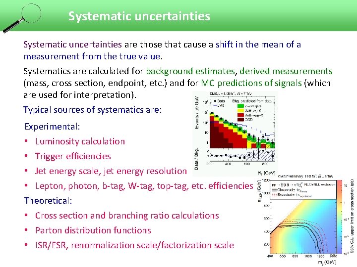
Systematic uncertainties are those that cause a shift in the mean of a measurement from the true value. Systematics are calculated for background estimates, derived measurements (mass, cross section, endpoint, etc. ) and for MC predictions of signals (which are used for interpretation). Typical sources of systematics are: Experimental: • Luminosity calculation • Trigger efficiencies • Jet energy scale, jet energy resolution • Lepton, photon, b-tag, W-tag, top-tag, etc. efficiencies Theoretical: • Cross section and branching ratio calculations • Parton distribution functions • ISR/FSR, renormalization scale/factorization scale 38

SUSY searches at CMS in other words “how we couldn’t yet find SUSY yet” 39

What is going on in CMS SUSY now? Most up-to-date public CMS SUSY results are listed here: https: //twiki. cern. ch/twiki/bin/view/CMSPublic/Physics. Results. SUS • Inclusive / generic searches: target mostly gluinos and 1 st/2 nd generation squarks • in this talk, S. Paktinat’s and E. Eskandari’s talks • Naturalness-inspired searches: targeting light stops/sbottoms and light gluinos with 3 rd generation decay modes • in S. Paktinat’s talk • Search for pair production of electroweak gauginos and sleptons • in H. Bakshian’s and A. Fahim’s talks • Search for Higgs in SUSY decays • in this talk • Search for multi-leptons and R-parity violating signatures • in B. Safarzadeh’s talk 40

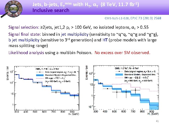
Jets, b-jets, ETmiss with HT, αT (8 Te. V, 11. 7 fb-1) Inclusive search CMS-SUS-12 -028, EPJC 73 (2013) 2568 Signal selection: ≥ 2 jets, jet 1, 2 p. T > 100 Ge. V, no isolated leptons, αT > 0. 55 Signal final state: binned in jet multiplicity (sensitivity to ~q~q, ~q~g and ~g~g), b jet multiplicity (sensitive to 3 rd generation) and HT (probe models with large mass splitting range) Likelihood analysis using a multibin Poisson. No excess over SM observed. 41

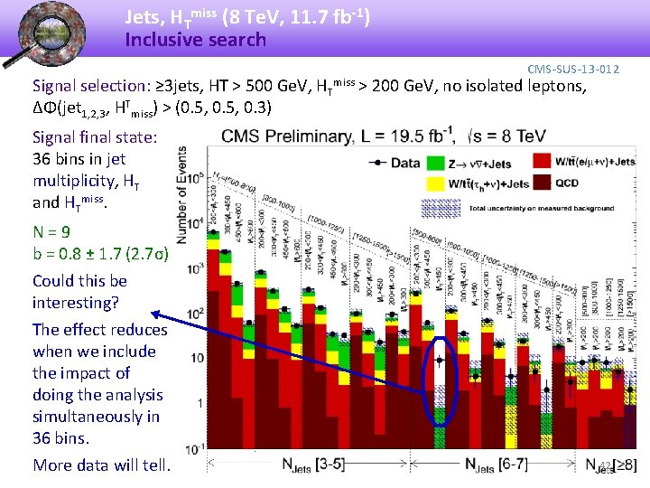
Jets, HTmiss (8 Te. V, 11. 7 fb-1) Inclusive search Signal selection: ≥ 3 jets, HT > 500 Ge. V, ΔΦ(jet 1, 2, 3, HTmiss) > (0. 5, 0. 3) HTmiss CMS-SUS-13 -012 > 200 Ge. V, no isolated leptons, Signal final state: 36 bins in jet multiplicity, HT and HTmiss. N=9 b = 0. 8 ± 1. 7 (2. 7σ) Could this be interesting? The effect reduces when we include the impact of doing the analysis simultaneously in 36 bins. More data will tell. 42

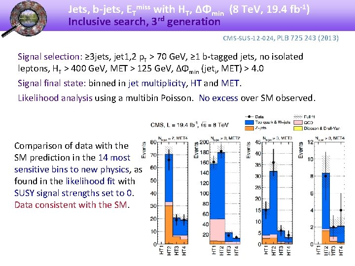
Jets, b-jets, ETmiss with HT, ΔΦmin (8 Te. V, 19. 4 fb-1) Inclusive search, 3 rd generation CMS-SUS-12 -024, PLB 725 243 (2013) Signal selection: ≥ 3 jets, jet 1, 2 p. T > 70 Ge. V, ≥ 1 b-tagged jets, no isolated leptons, HT > 400 Ge. V, MET > 125 Ge. V, ΔΦmin (jeti, MET) > 4. 0 Signal final state: binned in jet multiplicity, HT and MET. Likelihood analysis using a multibin Poisson. No excess over SM observed. Comparison of data with the SM prediction in the 14 most sensitive bins to new physics, as found in the likelihood fit with SUSY signal strengths set to 0. Data consistent with the SM. 43

Anomolous production of multileptons - I Inclusive search Signal selection: CMS-SUS-13 -002 3 or 4 leptons (e/μ) with possibly one tau with p. T > 20 Ge. V among them 0 or >1 b tagged jet HT < 200 Ge. V or > 200 Ge. V 0, 1 or 2 opposite-sign-same-flavor (OSSF) lepton pairs If OSSF exist: dilepton invariant mass mll below/on/above Z mass. Reject events with mll < 12 Ge. V to avoid low mass resonances. Reject events with both |ml+l- - m. Z| > 15 Ge. V and |ml+l-l’ – m. Z| < 15 Ge. V to avoid photon conversion from final state radiation. Signal final states: MET distributions in 64 bins of number of leptons, OSSF pairs, b-tagged jets, taus; dilepton mass wrt Z-mass and HT. Backgrounds: • ttbar, WZ smear MC MET distributions using data • non-prompt leptons or taus find conversion factor from data • asymmetric internal photon conversions find conversion factor from data 44 • •

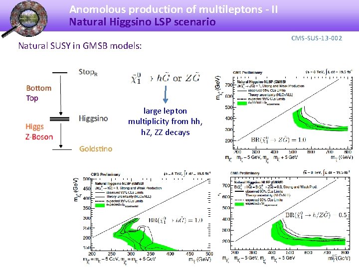
Anomolous production of multileptons - II Natural Higgsino LSP scenario Natural SUSY in GMSB models: CMS-SUS-13 -002 large lepton multiplicity from hh, h. Z, ZZ decays 45

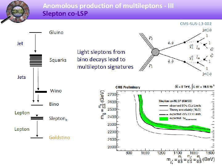
Anomolous production of multileptons - III Slepton co-LSP CMS-SUS-13 -002 Light sleptons from bino decays lead to multilepton signatures 46

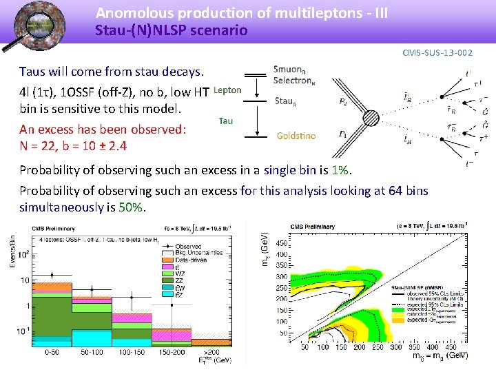
Anomolous production of multileptons - III Stau-(N)NLSP scenario CMS-SUS-13 -002 Taus will come from stau decays. 4 l (1τ), 1 OSSF (off-Z), no b, low HT bin is sensitive to this model. An excess has been observed: N = 22, b = 10 ± 2. 4 Probability of observing such an excess in a single bin is 1%. Probability of observing such an excess for this analysis looking at 64 bins simultaneously is 50%. 47

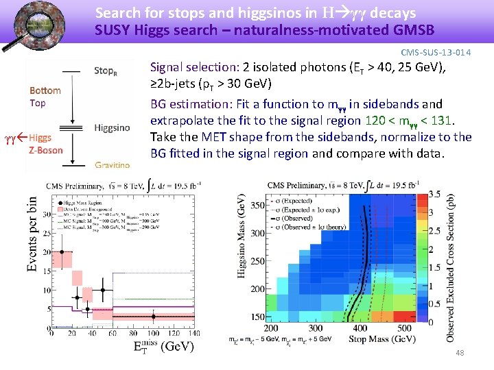
Search for stops and higgsinos in H γγ decays SUSY Higgs search – naturalness-motivated GMSB CMS-SUS-13 -014 γγ Signal selection: 2 isolated photons (ET > 40, 25 Ge. V), ≥ 2 b-jets (p. T > 30 Ge. V) BG estimation: Fit a function to mγγ in sidebands and extrapolate the fit to the signal region 120 < mγγ < 131. Take the MET shape from the sidebands, normalize to the BG fitted in the signal region and compare with data. 48

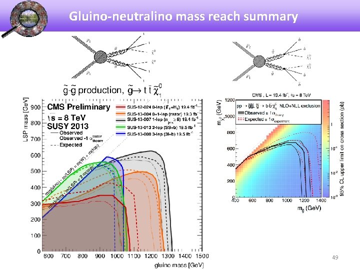
Gluino-neutralino mass reach summary 49

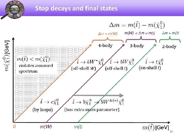
Stop decays and final states 50

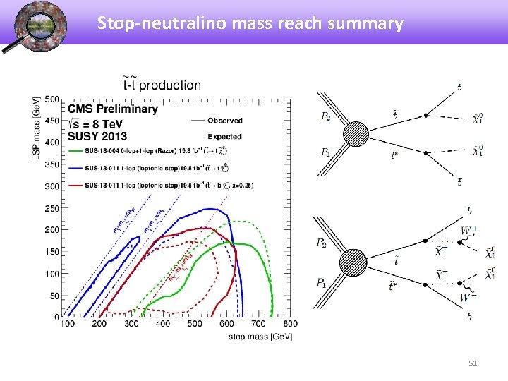
Stop-neutralino mass reach summary 51

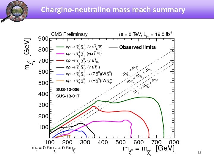
Chargino-neutralino mass reach summary 52

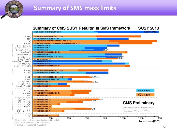
Summary of SMS mass limits 53

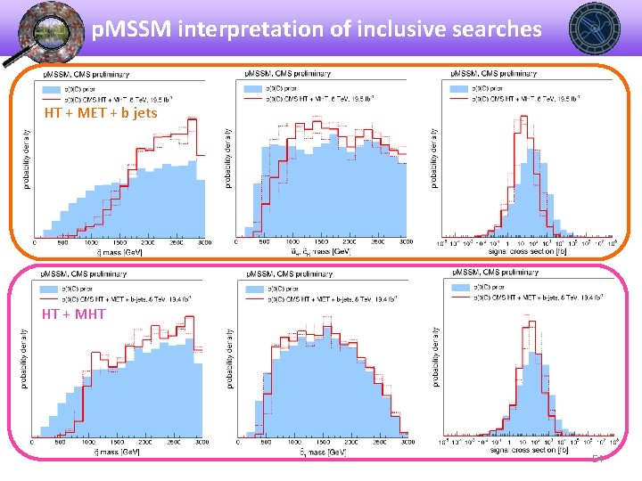
p. MSSM interpretation of inclusive searches HT + MET + b jets HT + MHT 54

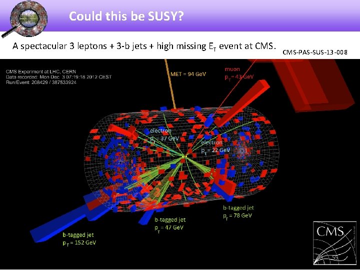
Could this be SUSY? A spectacular 3 leptons + 3 -b jets + high missing ET event at CMS-PAS-SUS-13 -008 55

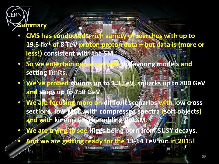
Summary • CMS has conducted a rich variety of searches with up to 19. 5 fb-1 of 8 Te. V proton data – but data is (more or less!) consistent with the SM. • So we entertain ourselves with disfavoring models and setting limits. • We've probed gluinos up to 1. 3 Te. V, squarks up to 800 Ge. V and stops up to 750 Ge. V. • We are focusing more on difficult scenarios with low cross sections, low MET, with compressed spectra (soft objects) and with kinematics resembling the SM. • We are trying to see Higgs being born from SUSY decays. • And we are getting ready for the 13 -14 Te. V run in 2015! 56

57

KEEP CALM AND SEARCH ON 58

BACKUP SLIDES 59

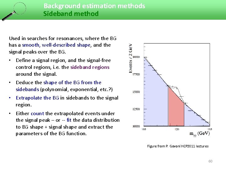
Background estimation methods Sideband method Used in searches for resonances, where the BG has a smooth, well-described shape, and the signal peaks over the BG. • Define a signal region, and the signal-free control regions, i. e. the sideband regions around the signal. • Deduce the shape of the BG from the sidebands (polynomial, exponential, etc. ? ) • Extrapolate the BG in sidebands to the signal region. • Either count the extrapolated events under the signal peak – or -- fit the data distribution to BG shape + signal shape and extract the parameters of the BG function. Figure from P. Govoni HCP 2011 lectures 60

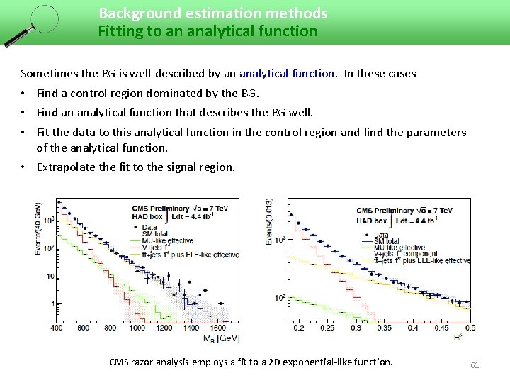
Background estimation methods Fitting to an analytical function Sometimes the BG is well-described by an analytical function. In these cases • Find a control region dominated by the BG. • Find an analytical function that describes the BG well. • Fit the data to this analytical function in the control region and find the parameters of the analytical function. • Extrapolate the fit to the signal region. CMS razor analysis employs a fit to a 2 D exponential-like function. 61

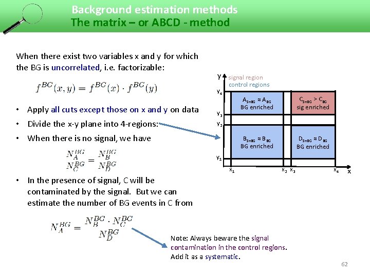
Background estimation methods The matrix – or ABCD - method When there exist two variables x and y for which the BG is uncorrelated, i. e. factorizable: y signal region y 4 • Apply all cuts except those on x and y on data • Divide the x-y plane into 4 -regions: • When there is no signal, we have control regions y 3 AS+BG ≈ ABG BG enriched CS+BG > CBG sig enriched BS+BG ≈ BBG BG enriched DS+BG ≈ DBG BG enriched y 2 y 1 x 2 x 3 • In the presence of signal, C will be contaminated by the signal. But we can estimate the number of BG events in C from Note: Always beware the signal contamination in the control regions. Add it as a systematic. x 4 x 62

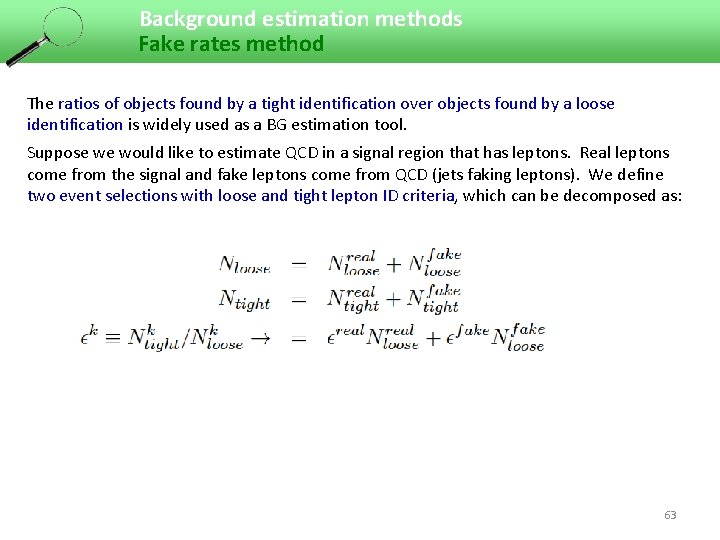
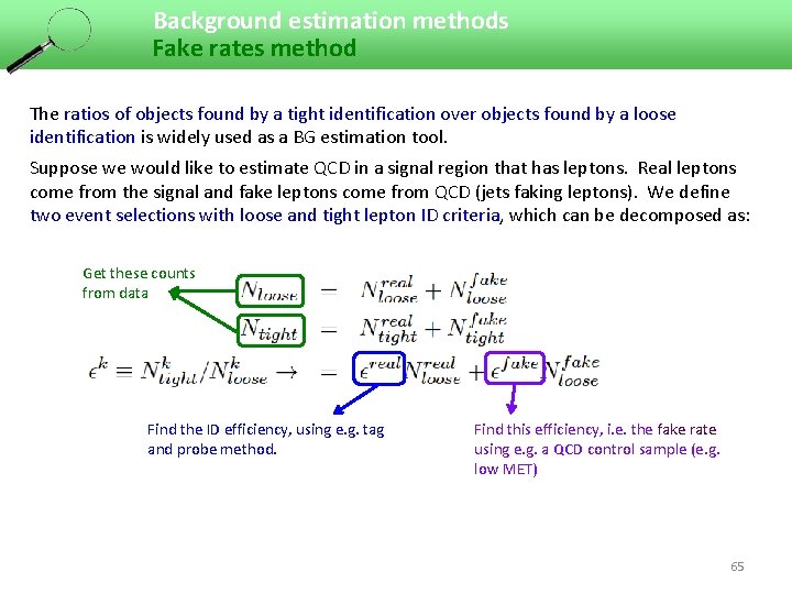
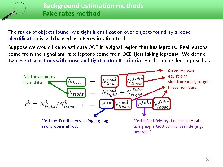
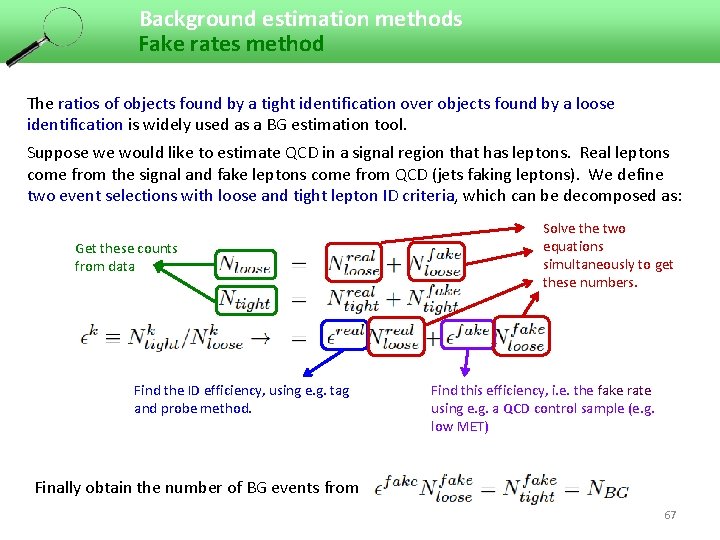
Background estimation methods Fake rates method The ratios of objects found by a tight identification over objects found by a loose identification is widely used as a BG estimation tool. Suppose we would like to estimate QCD in a signal region that has leptons. Real leptons come from the signal and fake leptons come from QCD (jets faking leptons). We define two event selections with loose and tight lepton ID criteria, which can be decomposed as: 63

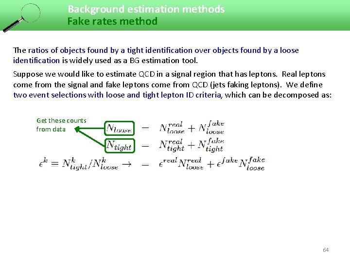
Background estimation methods Fake rates method The ratios of objects found by a tight identification over objects found by a loose identification is widely used as a BG estimation tool. Suppose we would like to estimate QCD in a signal region that has leptons. Real leptons come from the signal and fake leptons come from QCD (jets faking leptons). We define two event selections with loose and tight lepton ID criteria, which can be decomposed as: Get these counts from data 64

Background estimation methods Fake rates method The ratios of objects found by a tight identification over objects found by a loose identification is widely used as a BG estimation tool. Suppose we would like to estimate QCD in a signal region that has leptons. Real leptons come from the signal and fake leptons come from QCD (jets faking leptons). We define two event selections with loose and tight lepton ID criteria, which can be decomposed as: Get these counts from data Find the ID efficiency, using e. g. tag and probe method. Find this efficiency, i. e. the fake rate using e. g. a QCD control sample (e. g. low MET) 65

Background estimation methods Fake rates method The ratios of objects found by a tight identification over objects found by a loose identification is widely used as a BG estimation tool. Suppose we would like to estimate QCD in a signal region that has leptons. Real leptons come from the signal and fake leptons come from QCD (jets faking leptons). We define two event selections with loose and tight lepton ID criteria, which can be decomposed as: Get these counts from data Find the ID efficiency, using e. g. tag and probe method. Solve the two equations simultaneously to get these numbers. Find this efficiency, i. e. the fake rate using e. g. a QCD control sample (e. g. low MET) 66

Background estimation methods Fake rates method The ratios of objects found by a tight identification over objects found by a loose identification is widely used as a BG estimation tool. Suppose we would like to estimate QCD in a signal region that has leptons. Real leptons come from the signal and fake leptons come from QCD (jets faking leptons). We define two event selections with loose and tight lepton ID criteria, which can be decomposed as: Get these counts from data Find the ID efficiency, using e. g. tag and probe method. Solve the two equations simultaneously to get these numbers. Find this efficiency, i. e. the fake rate using e. g. a QCD control sample (e. g. low MET) Finally obtain the number of BG events from 67

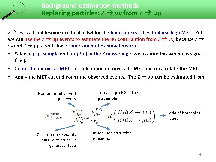
Background estimation methods Replacing particles: Z νν from Z μμ Z νν is a troublesome irreducible BG for the hadronic searches that use high MET. But we can use the Z μμ events to estimate the BG contribution from Z νν, because Z νν and Z μμ events have same kinematic characteristics. • Select a μ+μ- sample with m(μ+μ-) in the Z mass range (we assume this sample is signalfree). • Count the muons as MET, i. e. : add muon momenta to MET and recalculate the MET. • Apply the MET cut and count the observed events. The Z μμ can be estimated from Number of observed μμ events non-Z μμ BG in the μμ sample ratio of branching ratios Z mumu selected / total Z mumu in generator level muon reconstruction efficiency 68

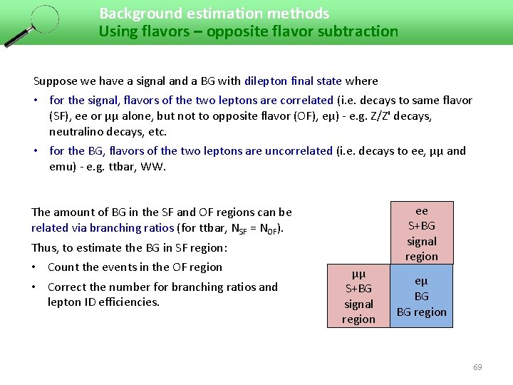
Background estimation methods Using flavors – opposite flavor subtraction Suppose we have a signal and a BG with dilepton final state where • for the signal, flavors of the two leptons are correlated (i. e. decays to same flavor (SF), ee or μμ alone, but not to opposite flavor (OF), eμ) - e. g. Z/Z' decays, neutralino decays, etc. • for the BG, flavors of the two leptons are uncorrelated (i. e. decays to ee, μμ and emu) - e. g. ttbar, WW. ee S+BG signal region The amount of BG in the SF and OF regions can be related via branching ratios (for ttbar, NSF = NOF). Thus, to estimate the BG in SF region: • Count the events in the OF region • Correct the number for branching ratios and lepton ID efficiencies. μμ S+BG signal region eμ BG BG region 69