Search Tuomas Sandholm Read Russell Norvig Sections 3

Search Tuomas Sandholm Read Russell & Norvig Sections 3. 1 -3. 4. (Also read Chapters 1 and 2 if you haven’t already. ) Minor additions by Dave Touretzky in 2018 1

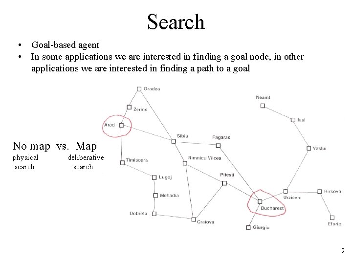
Search • • Goal-based agent In some applications we are interested in finding a goal node, in other applications we are interested in finding a path to a goal No map vs. Map physical search deliberative search 2

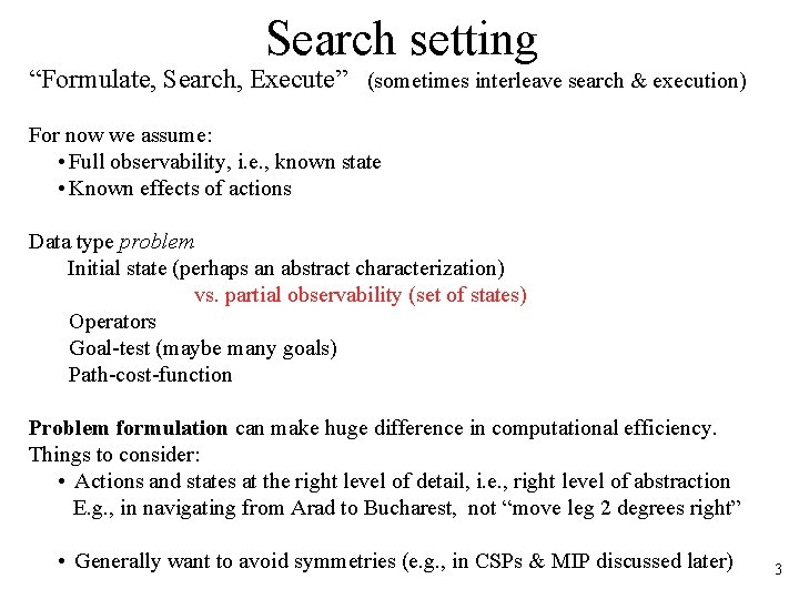
Search setting “Formulate, Search, Execute” (sometimes interleave search & execution) For now we assume: • Full observability, i. e. , known state • Known effects of actions Data type problem Initial state (perhaps an abstract characterization) vs. partial observability (set of states) Operators Goal-test (maybe many goals) Path-cost-function Problem formulation can make huge difference in computational efficiency. Things to consider: • Actions and states at the right level of detail, i. e. , right level of abstraction E. g. , in navigating from Arad to Bucharest, not “move leg 2 degrees right” • Generally want to avoid symmetries (e. g. , in CSPs & MIP discussed later) 3

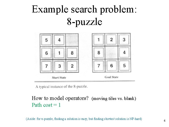
Example search problem: 8 -puzzle How to model operators? (moving tiles vs. blank) Path cost = 1 (Aside: for n-puzzle, finding a solution is easy, but finding shortest solution is NP-hard) 4

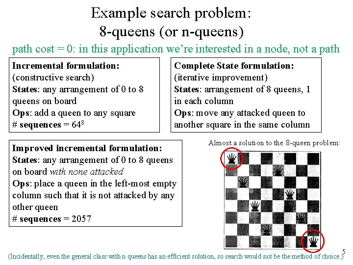
Example search problem: 8 -queens (or n-queens) path cost = 0: in this application we’re interested in a node, not a path Incremental formulation: (constructive search) States: any arrangement of 0 to 8 queens on board Ops: add a queen to any square # sequences = 648 Complete State formulation: (iterative improvement) States: arrangement of 8 queens, 1 in each column Ops: move any attacked queen to another square in the same column Improved incremental formulation: States: any arrangement of 0 to 8 queens on board with none attacked Ops: place a queen in the left-most empty column such that it is not attacked by any other queen # sequences = 2057 Almost a solution to the 8 -queen problem: 5 (Incidentally, even the general class with n queens has an efficient solution, so search would not be the method of choice. )

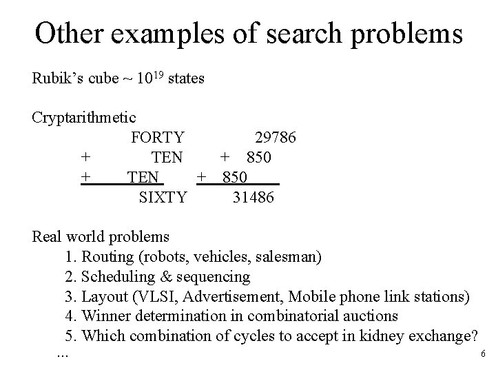
Other examples of search problems Rubik’s cube ~ 1019 states Cryptarithmetic FORTY 29786 + TEN + 850 + TEN + 850 SIXTY 31486 Real world problems 1. Routing (robots, vehicles, salesman) 2. Scheduling & sequencing 3. Layout (VLSI, Advertisement, Mobile phone link stations) 4. Winner determination in combinatorial auctions 5. Which combination of cycles to accept in kidney exchange? … 6

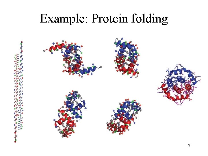
Example: Protein folding 7

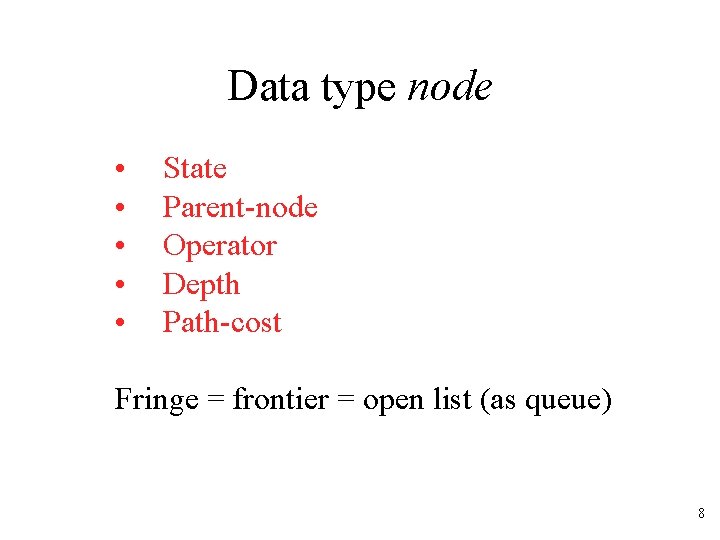
Data type node • State • Parent-node • Operator • Depth • Path-cost Fringe = frontier = open list (as queue) 8

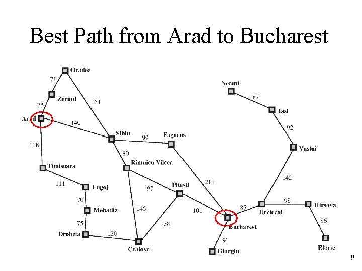
Best Path from Arad to Bucharest 9

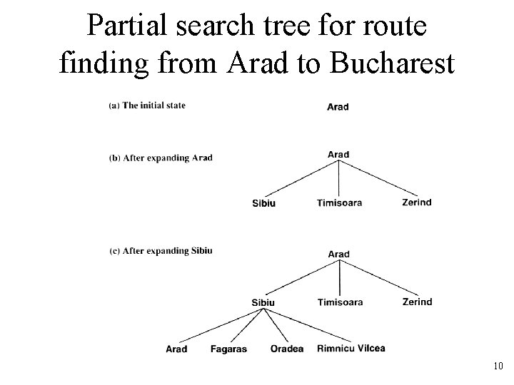
Partial search tree for route finding from Arad to Bucharest 10

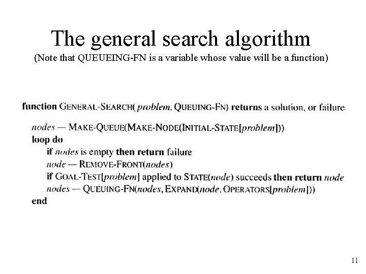
The general search algorithm (Note that QUEUEING-FN is a variable whose value will be a function) 11

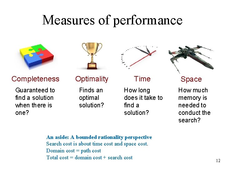
Measures of performance Completeness Optimality Time Guaranteed to find a solution when there is one? Finds an optimal solution? How long does it take to find a solution? An aside: A bounded rationality perspective Search cost is about time cost and space cost. Domain cost = path cost Total cost = domain cost + search cost Space How much memory is needed to conduct the search? 12

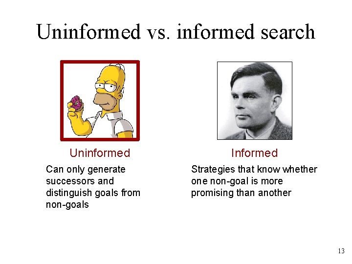
Uninformed vs. informed search Uninformed Can only generate successors and distinguish goals from non-goals Informed Strategies that know whether one non-goal is more promising than another 13

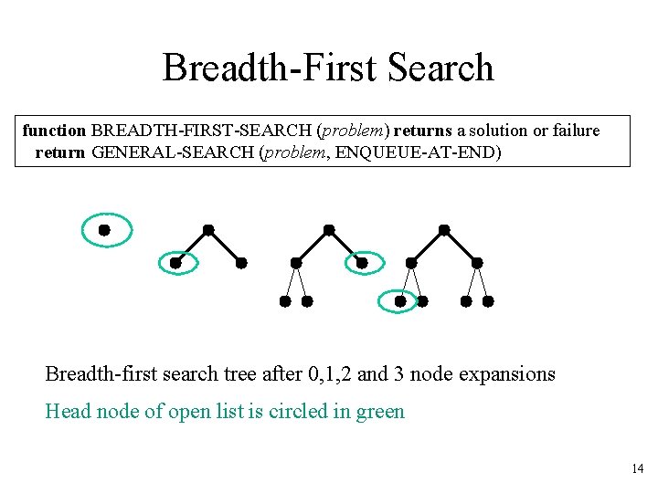
Breadth-First Search function BREADTH-FIRST-SEARCH (problem) returns a solution or failure return GENERAL-SEARCH (problem, ENQUEUE-AT-END) Breadth-first search tree after 0, 1, 2 and 3 node expansions Head node of open list is circled in green 14

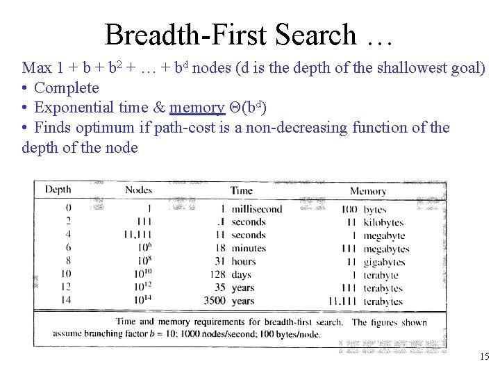
Breadth-First Search … Max 1 + b 2 + … + bd nodes (d is the depth of the shallowest goal) • Complete • Exponential time & memory Θ(bd) • Finds optimum if path-cost is a non-decreasing function of the depth of the node 15

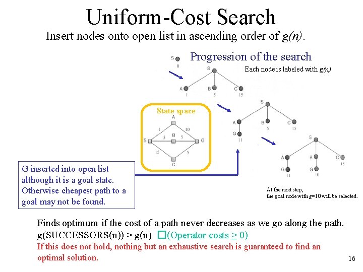
Uniform-Cost Search Insert nodes onto open list in ascending order of g(n). Progression of the search Each node is labeled with g(n) State space G inserted into open list although it is a goal state. Otherwise cheapest path to a goal may not be found. At the next step, the goal node with g=10 will be selected. Finds optimum if the cost of a path never decreases as we go along the path. g(SUCCESSORS(n)) ≥ g(n) � (Operator costs ≥ 0) If this does not hold, nothing but an exhaustive search is guaranteed to find an optimal solution. 16

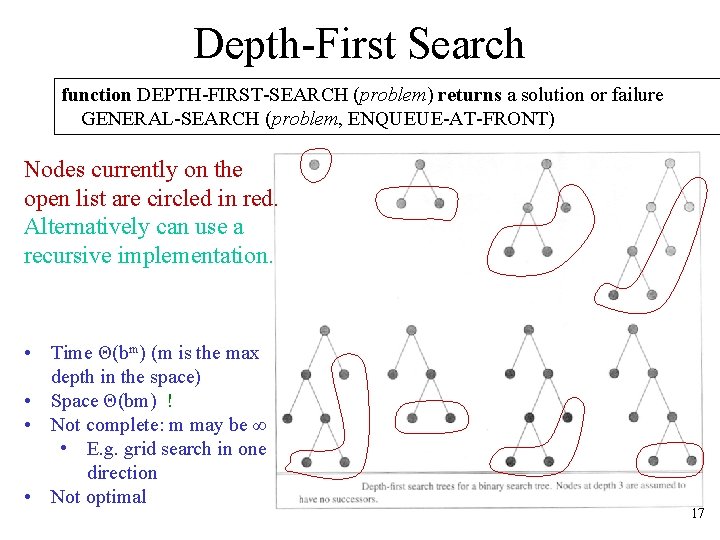
Depth-First Search function DEPTH-FIRST-SEARCH (problem) returns a solution or failure GENERAL-SEARCH (problem, ENQUEUE-AT-FRONT) Nodes currently on the open list are circled in red. Alternatively can use a recursive implementation. • • Time Θ(bm) (m is the max depth in the space) Space Θ(bm) ! Not complete: m may be ∞ • E. g. grid search in one direction Not optimal 17

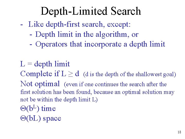
Depth-Limited Search - Like depth-first search, except: - Depth limit in the algorithm, or - Operators that incorporate a depth limit L = depth limit Complete if L ≥ d (d is the depth of the shallowest goal) Not optimal (even if one continues the search after the first solution has been found, because an optimal solution may not be within the depth limit L) Θ(b. L) time Θ(b. L) space 18

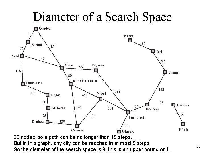
Diameter of a Search Space 20 nodes, so a path can be no longer than 19 steps. But in this graph, any city can be reached in at most 9 steps. So the diameter of the search space is 9; this is an upper bound on L. 19

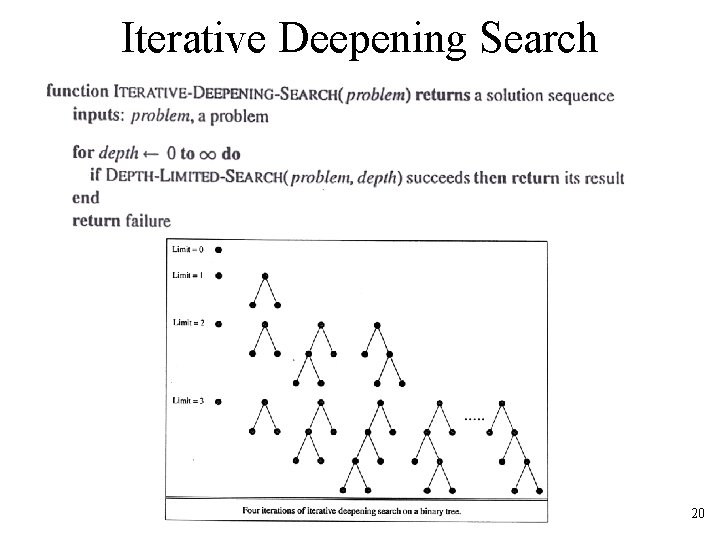
Iterative Deepening Search 20

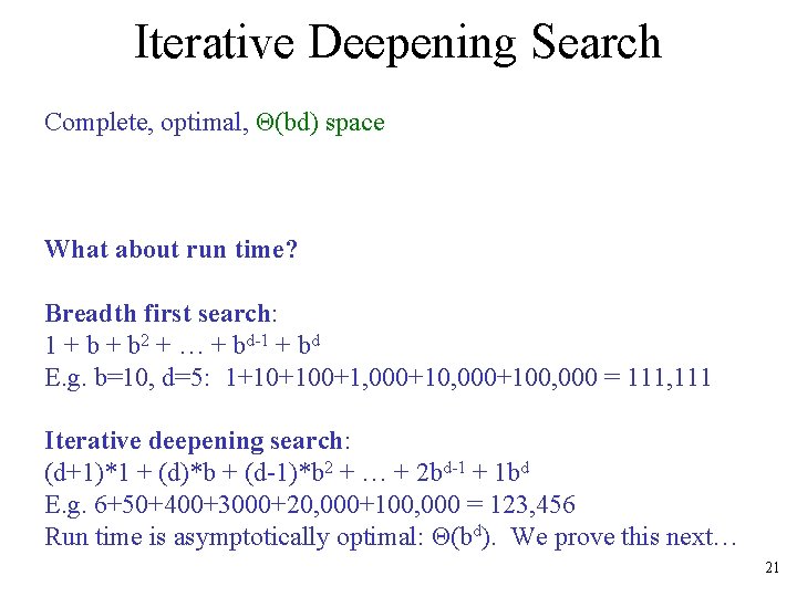
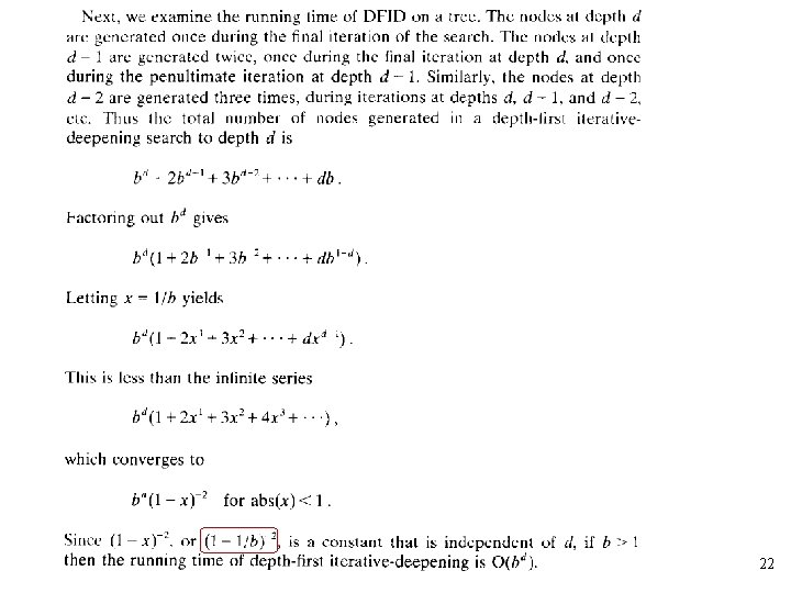
Iterative Deepening Search Complete, optimal, Θ(bd) space What about run time? Breadth first search: 1 + b 2 + … + bd-1 + bd E. g. b=10, d=5: 1+10+100+1, 000+100, 000 = 111, 111 Iterative deepening search: (d+1)*1 + (d)*b + (d-1)*b 2 + … + 2 bd-1 + 1 bd E. g. 6+50+400+3000+20, 000+100, 000 = 123, 456 Run time is asymptotically optimal: Θ(bd). We prove this next… 21

22

Question Is iterative deepening preferred when branching factor is small or large? 23

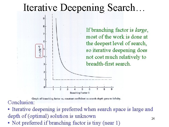
Iterative Deepening Search… If branching factor is large, most of the work is done at the deepest level of search, so iterative deepening does not cost much relatively to breadth-first search. Conclusion: • Iterative deepening is preferred when search space is large and depth of (optimal) solution is unknown 24 • Not preferred if branching factor is tiny (near 1)

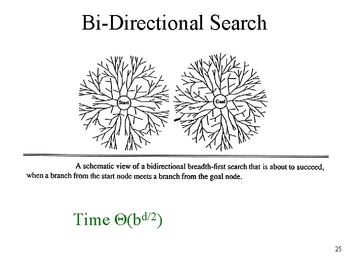
Bi-Directional Search Time Θ(bd/2) 25

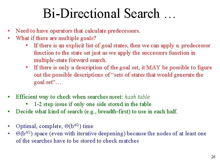
Bi-Directional Search … • • Need to have operators that calculate predecessors. What if there are multiple goals? • If there is an explicit list of goal states, then we can apply a predecessor function to the state set just as we apply the successors function in multiple-state forward search. • If there is only a description of the goal set, it MAY be possible to figure out the possible descriptions of “sets of states that would generate the goal set”… • Efficient way to check when searches meet: hash table • 1 -2 step issue if only one side stored in the table Decide what kind of search (e. g. , breadth-first) to use in each half. • • • Optimal, complete, Θ(bd/2) time Θ(bd/2) space (even with iterative deepening) because the nodes of at least one of the searches have to be stored to check matches 26

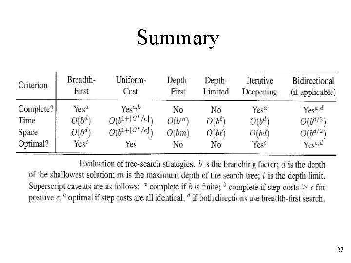
Summary 27

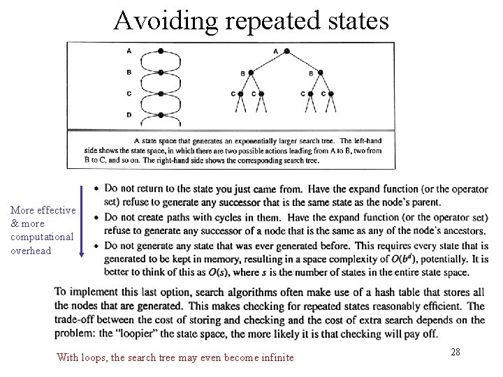
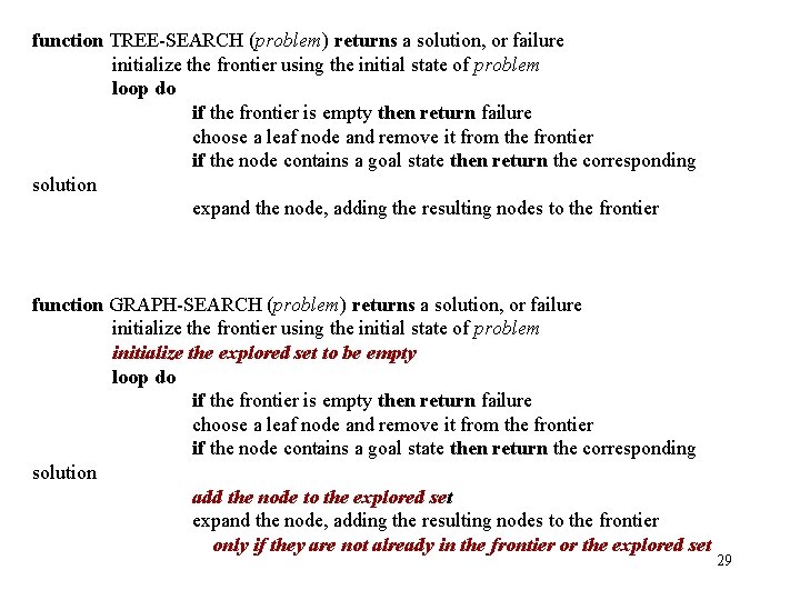
Avoiding repeated states More effective & more computational overhead With loops, the search tree may even become infinite 28

function TREE-SEARCH (problem) returns a solution, or failure initialize the frontier using the initial state of problem loop do if the frontier is empty then return failure choose a leaf node and remove it from the frontier if the node contains a goal state then return the corresponding solution expand the node, adding the resulting nodes to the frontier function GRAPH-SEARCH (problem) returns a solution, or failure initialize the frontier using the initial state of problem initialize the explored set to be empty loop do if the frontier is empty then return failure choose a leaf node and remove it from the frontier if the node contains a goal state then return the corresponding solution add the node to the explored set expand the node, adding the resulting nodes to the frontier only if they are not already in the frontier or the explored set 29

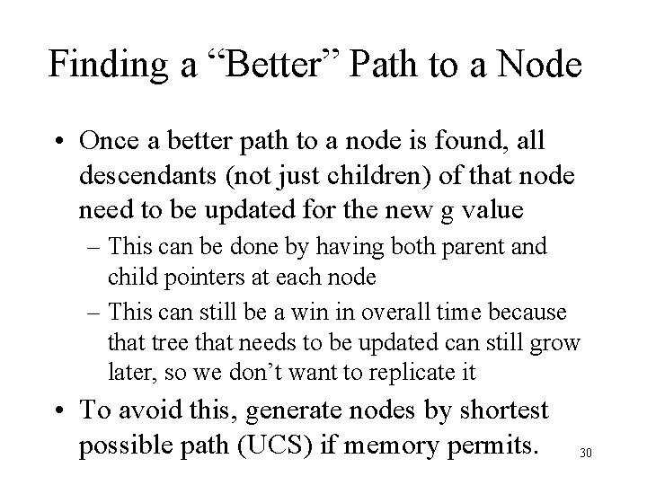
Finding a “Better” Path to a Node • Once a better path to a node is found, all descendants (not just children) of that node need to be updated for the new g value – This can be done by having both parent and child pointers at each node – This can still be a win in overall time because that tree that needs to be updated can still grow later, so we don’t want to replicate it • To avoid this, generate nodes by shortest possible path (UCS) if memory permits. 30

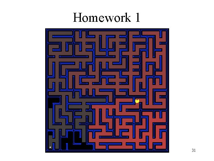
Homework 1 31