Search Trees CSE 2320 Algorithms and Data Structures

Search Trees CSE 2320 – Algorithms and Data Structures Alexandra Stefan Based on slides and notes from: Vassilis Athitsos and Bob Weems University of Texas at Arlington 3/4/2021 1

Search Trees • Preliminary note: "search trees" as a term does NOT refer to a specific implementation. • The term refers to a family of implementations, that may have different properties. • We will discuss: – Binary search trees (BST). – 2 -3 -4 trees (a special type of a B-tree). – Other trees: red-black trees, AVL trees, splay trees, B-trees and other variations. 2

Search Trees • All search trees support search, insertion and deletion operations. • Insertions and deletions can differ among trees, and have important implications on overall performance. • The main goal is to have insertions and deletions that: – Are efficient (at most logarithmic time). – Leave the tree balanced, to support efficient search (at most logarithmic time). 3

Binary Search Trees (BST) 4

Binary Search Tree (BST) • Resources: – BST in general – CLRS – BST in general and solved problems: http: //cslibrary. stanford. edu/110/Binary. Trees. html#s – Insertion at root (using insertion at a leaf and rotations) • Sedgewick • Dr. Bob Weems: Notes 11, parts: ‘ 11. D. Rotations’ and ’ 11. E. Insertion At Root’ – Randomizing the tree by inserting at a random position: • Sedgewick 5

Tree Properties - Review • Full tree • Complete tree (e. g. heap tree) • Perfect binary tree • Alternative definitions: complete (for perfect) and almost complete or nearly complete (complete). • Tree – connected graph with no cycles, or connected graph with N-1 edges (and N vertices). 6

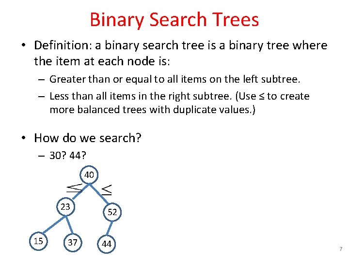
Binary Search Trees • Definition: a binary search tree is a binary tree where the item at each node is: – Greater than or equal to all items on the left subtree. – Less than all items in the right subtree. (Use ≤ to create more balanced trees with duplicate values. ) • How do we search? – 30? 44? 40 23 15 37 52 44 7

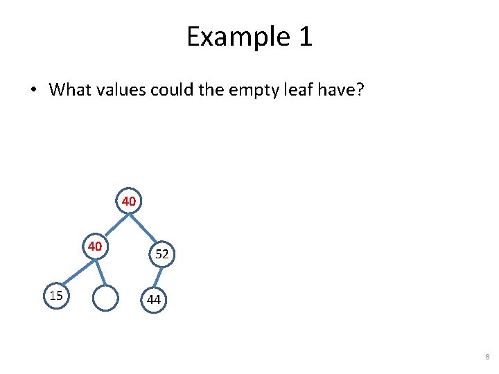
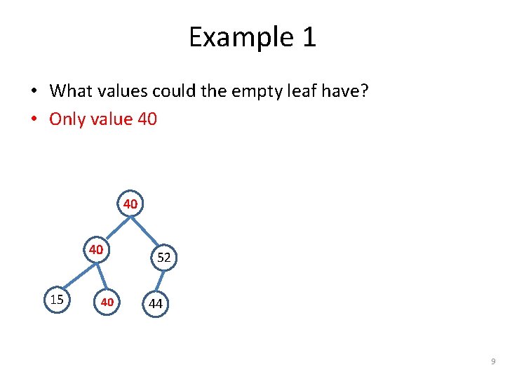
Example 1 • What values could the empty leaf have? 40 40 15 52 44 8

Example 1 • What values could the empty leaf have? • Only value 40 40 40 15 40 52 44 9

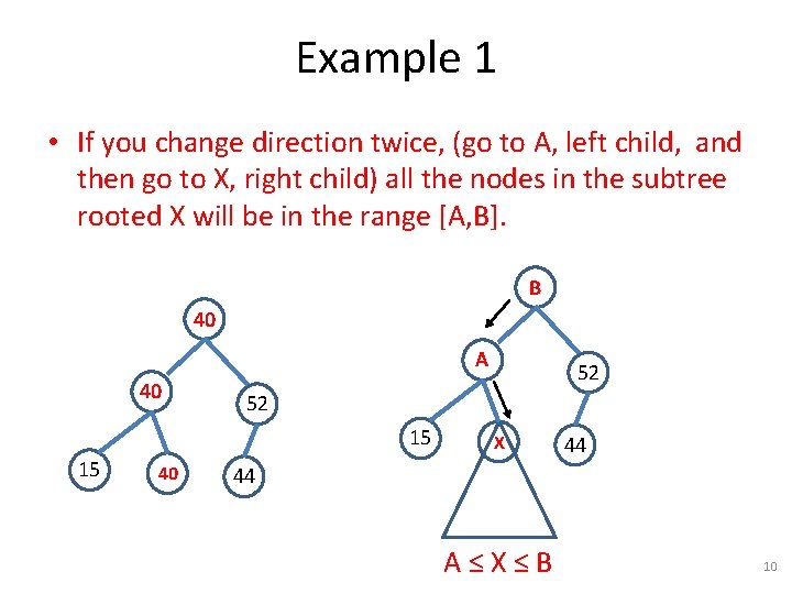
Example 1 • If you change direction twice, (go to A, left child, and then go to X, right child) all the nodes in the subtree rooted X will be in the range [A, B]. B 40 A 40 52 15 15 40 52 X 44 44 A≤X≤B 10

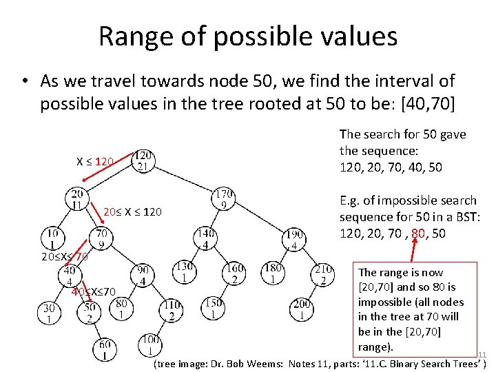
Range of possible values • As we travel towards node 50, we find the interval of possible values in the tree rooted at 50 to be: [40, 70] The search for 50 gave the sequence: 120, 70, 40, 50 X ≤ 120 20≤ X ≤ 120 E. g. of impossible search sequence for 50 in a BST: 120, 70 , 80, 50 20≤X≤ 70 40≤X≤ 70 The range is now [20, 70] and so 80 is impossible (all nodes in the tree at 70 will be in the [20, 70] range). 11 (tree image: Dr. Bob Weems: Notes 11, parts: ‘ 11. C. Binary Search Trees’ )

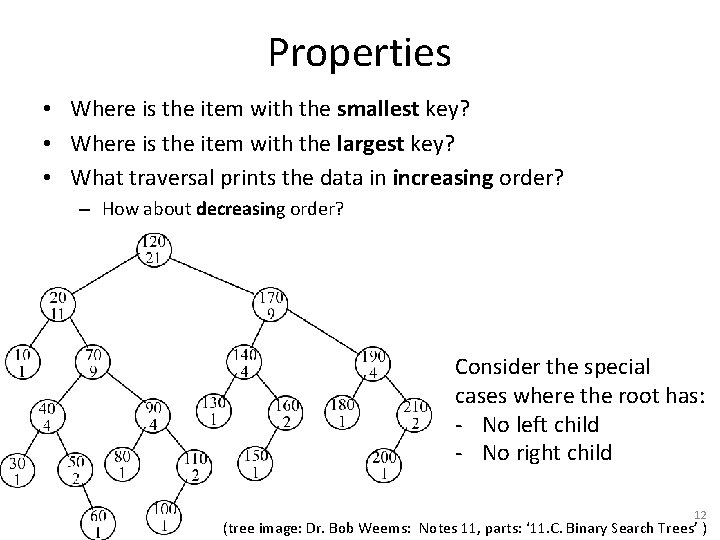
Properties • Where is the item with the smallest key? • Where is the item with the largest key? • What traversal prints the data in increasing order? – How about decreasing order? Consider the special cases where the root has: - No left child - No right child 12 (tree image: Dr. Bob Weems: Notes 11, parts: ‘ 11. C. Binary Search Trees’ )

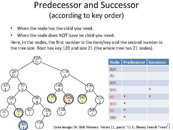
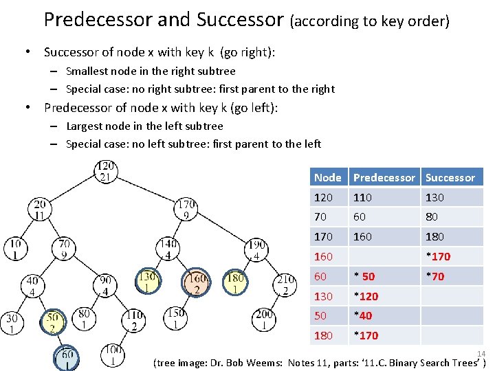
Predecessor and Successor (according to key order) • When the node has the child you need. • When the node does NOT have he child you need. Here, in the nodes, the first number is the item/key and the second number is the tree size. Root has key 120 and size 21 (the whole tree has 21 nodes). Node Predecessor Successor 120 70 160 * 130 * 50 * 180 * * 13 (tree image: Dr. Bob Weems: Notes 11, parts: ‘ 11. C. Binary Search Trees’ )

Predecessor and Successor (according to key order) • Successor of node x with key k (go right): – Smallest node in the right subtree – Special case: no right subtree: first parent to the right • Predecessor of node x with key k (go left): – Largest node in the left subtree – Special case: no left subtree: first parent to the left Node Predecessor Successor 120 110 130 70 60 80 170 160 180 160 *170 60 * 50 130 *120 50 *40 180 *170 *70 14 (tree image: Dr. Bob Weems: Notes 11, parts: ‘ 11. C. Binary Search Trees’ )

• Min: leftmost node (from the root keep going left) – Special case: no left child => root • Max: rightmost node (from the root keep going right. – Special case: no right child => root • Print in order: – Increasing: Left, Root, Right (inorder traversal) – Decreasing: Right, Root, Left • Successor of node x with key k (go right): – Smallest node in the right subtree – Special case: no right subtree: first parent to the right • Predecessor of node x with key k (go left): – Largest node in the left subtree – Special case: no left subtree: first parent to the left 15

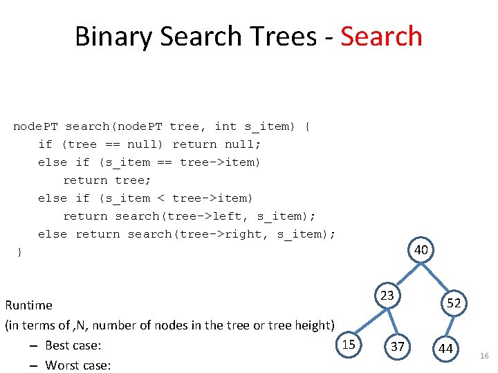
Binary Search Trees - Search node. PT search(node. PT tree, int s_item) { if (tree == null) return null; else if (s_item == tree->item) return tree; else if (s_item < tree->item) return search(tree->left, s_item); else return search(tree->right, s_item); } Runtime (in terms of , N, number of nodes in the tree or tree height) 15 – Best case: – Worst case: 40 23 37 52 44 16

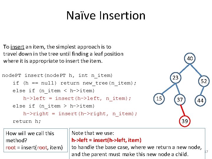
Naïve Insertion To insert an item, the simplest approach is to travel down in the tree until finding a leaf position where it is appropriate to insert the item. node. PT insert(node. PT h, int n_item) if (h == null) return new_tree(n_item); else if (n_item < h->item) h->left = insert(h->left, n_item); else if (n_item > h->item) h->right = insert(h->right, n_item); return h; How will we call this method? root = insert(root, item) 40 23 15 52 37 44 39 Note that we use: h->left = insert(h->left, item) to handle the base case, where we return a new node, and the parent must make this new node a child. 17

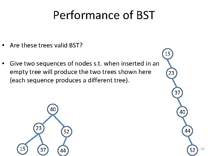
Performance of BST • Are these trees valid BST? 15 • Give two sequences of nodes s. t. when inserted in an empty tree will produce the two trees shown here (each sequence produces a different tree). 23 37 40 23 15 37 40 52 44 44 52 18

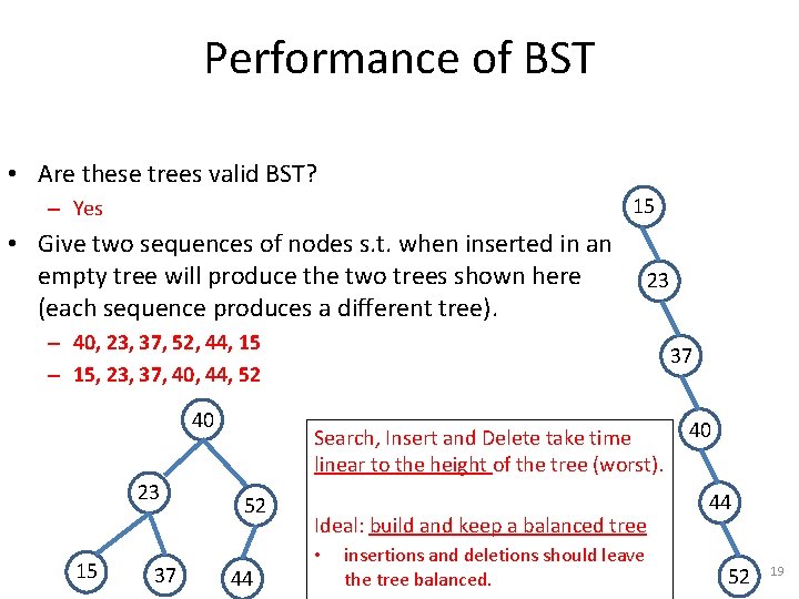
Performance of BST • Are these trees valid BST? 15 – Yes • Give two sequences of nodes s. t. when inserted in an empty tree will produce the two trees shown here (each sequence produces a different tree). 23 – 40, 23, 37, 52, 44, 15 – 15, 23, 37, 40, 44, 52 40 23 15 37 37 Search, Insert and Delete take time linear to the height of the tree (worst). 52 44 Ideal: build and keep a balanced tree • insertions and deletions should leave the tree balanced. 40 44 52 19

Performance of BST • If items are inserted in: – ascending order, the resulting tree is maximally imbalanced. – random order, the resulting trees are reasonably balanced. • Can we insert the items in random order? – If we build the tree from a batch of items. • Shuffle them first, or grab them from random positions. – If they come online (we do not have them all as a batch). • Insert in the tree at a random position 20

BST - Randomized • If the data can be inserted in random order, on average, the tree will be balanced. • If we do not have control over the data: insert at a RANDOM position in the tree – When inserting in tree of size N, • Insert at the root with probability 1/(N+1) – New tree size will be (N+1) • If not at the root, go to the appropriate subtree (e. g. go left if the key of new item is smaller or equal than that of the root item) and repeat the process. 21

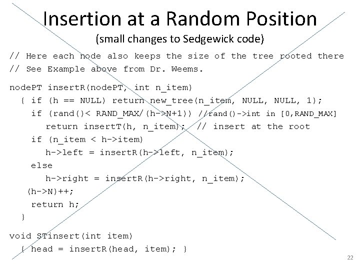
Insertion at a Random Position (small changes to Sedgewick code) // Here each node also keeps the size of the tree rooted there // See Example above from Dr. Weems. node. PT insert. R(node. PT, int n_item) { if (h == NULL) return new_tree(n_item, NULL, 1); if (rand()< RAND_MAX/(h->N+1)) //rand()->int in [0, RAND_MAX] return insert. T(h, n_item); // insert at the root if (n_item < h->item) h->left = insert. R(h->left, n_item); else h->right = insert. R(h->right, n_item); (h->N)++; return h; } void STinsert(int item) { head = insert. R(head, item); } 22

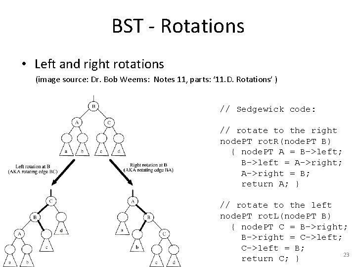
BST - Rotations • Left and right rotations (image source: Dr. Bob Weems: Notes 11, parts: ‘ 11. D. Rotations’ ) // Sedgewick code: // rotate to the right node. PT rot. R(node. PT B) { node. PT A = B->left; B->left = A->right; A->right = B; return A; } // rotate to the left node. PT rot. L(node. PT B) { node. PT C = B->right; B->right = C->left; C->left = B; 23 return C; }

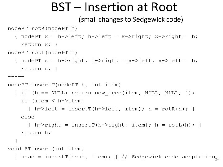
BST – Insertion at Root (small changes to Sedgewick code) node. PT rot. R(node. PT h) { node. PT x = h->left; h->left = x->right; x->right = h; return x; } node. PT rot. L(node. PT h) { node. PT x = h->right; h->right = x->left; x->left = h; return x; } ----node. PT insert. T(node. PT h, int item) { if (h == NULL) return new_tree(item, NULL, 1); if (item < h->item) { h->left = insert. T(h->left, item); h = rot. R(h); } else { h->right = insert. T(h->right, item); h = rot. L(h); } return h; } void STinsert(int item) { head = insert. T(head, item); } // Sedgewick code adaptation 24

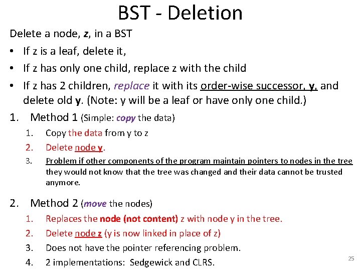
BST - Deletion Delete a node, z, in a BST • If z is a leaf, delete it, • If z has only one child, replace z with the child • If z has 2 children, replace it with its order-wise successor, y, and delete old y. (Note: y will be a leaf or have only one child. ) 1. Method 1 (Simple: copy the data) 1. 2. Copy the data from y to z Delete node y. 3. Problem if other components of the program maintain pointers to nodes in the tree they would not know that the tree was changed and their data cannot be trusted anymore. 2. Method 2 (move the nodes) 1. 2. 3. 4. Replaces the node (not content) z with node y in the tree. Delete node z (y is now linked in place of z) Does not have the pointer referencing problem. 2 implementations: Sedgewick and CLRS. 25

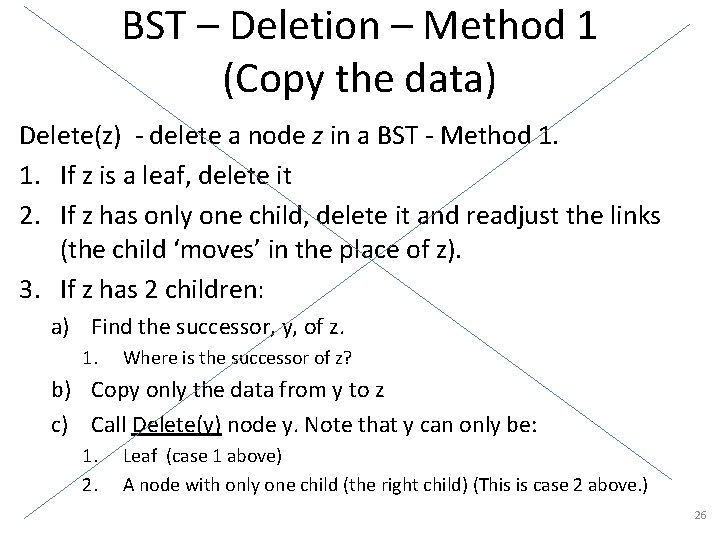
BST – Deletion – Method 1 (Copy the data) Delete(z) - delete a node z in a BST - Method 1. 1. If z is a leaf, delete it 2. If z has only one child, delete it and readjust the links (the child ‘moves’ in the place of z). 3. If z has 2 children: a) Find the successor, y, of z. 1. Where is the successor of z? b) Copy only the data from y to z c) Call Delete(y) node y. Note that y can only be: 1. 2. Leaf (case 1 above) A node with only one child (the right child) (This is case 2 above. ) 26

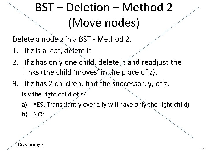
BST – Deletion – Method 2 (Move nodes) Delete a node z in a BST - Method 2. 1. If z is a leaf, delete it 2. If z has only one child, delete it and readjust the links (the child ‘moves’ in the place of z). 3. If z has 2 children, find the successor, y, of z. Is y the right child of z? a) YES: Transplant y over z (y will have only the right child) b) NO: Draw image 27

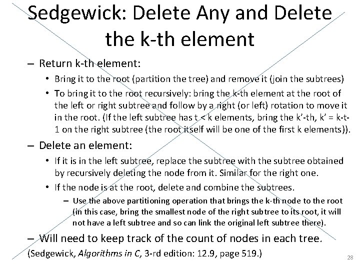
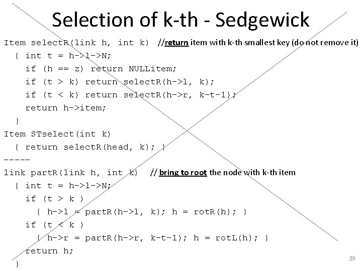
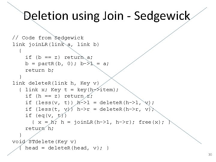
Sedgewick: Delete Any and Delete the k-th element – Return k-th element: • Bring it to the root (partition the tree) and remove it (join the subtrees) • To bring it to the root recursively: bring the k-th element at the root of the left or right subtree and follow by a right (or left) rotation to move it in the root. (If the left subtree has t < k elements, bring the k’-th, k’ = k-t 1 on the right subtree (the root itself will be one of the first k elements)). – Delete an element: • If it is in the left subtree, replace the subtree with the subtree obtained by recursively deleting the node from it. Similar for the right one. • If the node is at the root, delete and combine the subtrees. – Use the above partitioning operation that brings the k-th node to the root (in this case, bring the smallest node of the right subtree to its root, it will not have a left subtree and so can link the original left subtree there). – Will need to keep track of the count of nodes in each tree. (Sedgewick, Algorithms in C, 3 -rd edition: 12. 9, page 519. ) 28

Selection of k-th - Sedgewick Item select. R(link h, int k) //return item with k-th smallest key (do not remove it) { int t = h->l->N; if (h == z) return NULLitem; if (t > k) return select. R(h->l, k); if (t < k) return select. R(h->r, k-t-1); return h->item; } Item STselect(int k) { return select. R(head, k); } ----link part. R(link h, int k) // bring to root the node with k-th item { int t = h->l->N; if (t > k ) { h->l = part. R(h->l, k); h = rot. R(h); } if (t < k ) { h->r = part. R(h->r, k-t-1); h = rot. L(h); } return h; 29 }

Deletion using Join - Sedgewick // Code from Sedgewick link join. LR(link a, link b) { if (b == z) return a; b = part. R(b, 0); b->l = a; return b; } link delete. R(link h, Key v) { link x; Key t = key(h->item); if (h == z) return z; if (less(v, t)) h->l = delete. R(h->l, v); if (less(t, v)) h->r = delete. R(h->r, v); if (eq(v, t)) { x = h; h = join. LR(h->l, h->r); free(x); } return h; } void STdelete(Key v) { head = delete. R(head, v); } 30

2 -3 -4 Tree • Next we will see 2 -3 -4 tree, which is guaranteed to stay balanced regardless of the order of insertions. 31

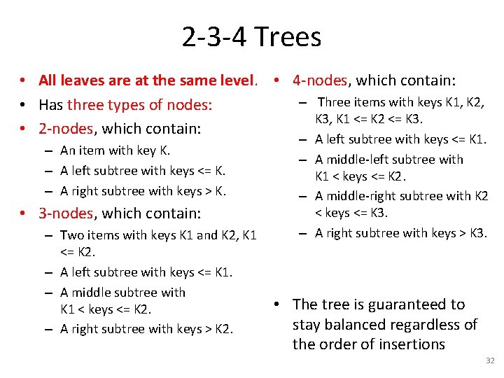
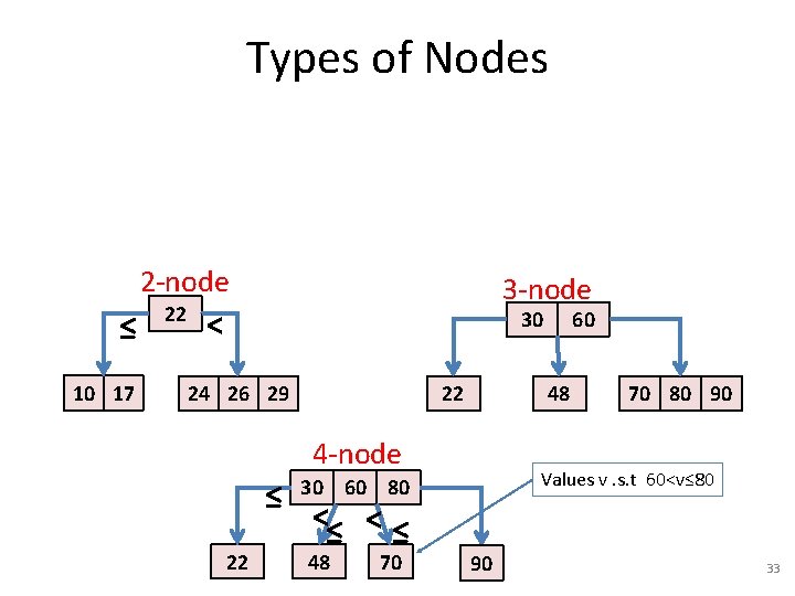
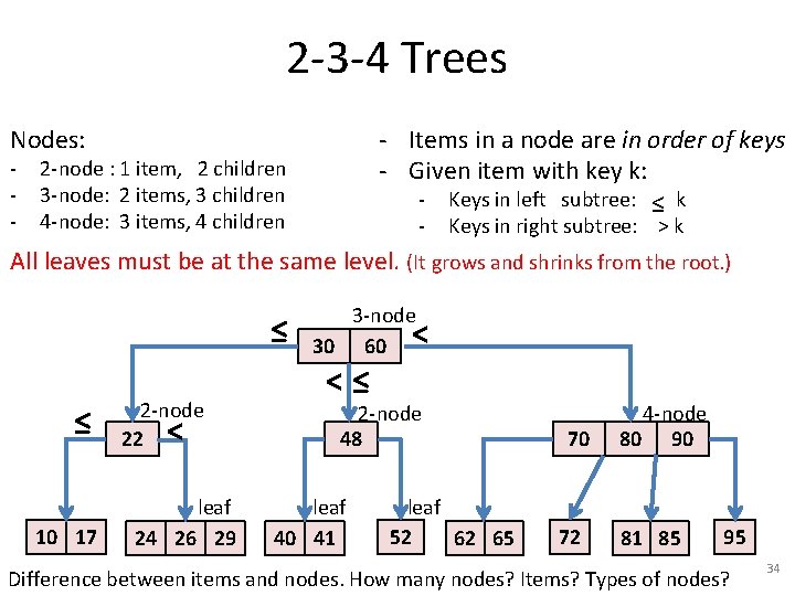
2 -3 -4 Trees • All leaves are at the same level. • 4 -nodes, which contain: – Three items with keys K 1, K 2, • Has three types of nodes: K 3, K 1 <= K 2 <= K 3. • 2 -nodes, which contain: – An item with key K. – A left subtree with keys <= K. – A right subtree with keys > K. • 3 -nodes, which contain: – Two items with keys K 1 and K 2, K 1 <= K 2. – A left subtree with keys <= K 1. – A middle subtree with K 1 < keys <= K 2. – A right subtree with keys > K 2. – A left subtree with keys <= K 1. – A middle-left subtree with K 1 < keys <= K 2. – A middle-right subtree with K 2 < keys <= K 3. – A right subtree with keys > K 3. • The tree is guaranteed to stay balanced regardless of the order of insertions 32

Types of Nodes 2 -node ≤ 10 17 22 3 -node < 30 24 26 29 22 48 4 -node ≤ 22 48 70 70 80 90 Values v. s. t 60<v≤ 80 30 60 80 <≤ < ≤ 60 90 33

2 -3 -4 Trees - Items in a node are in order of keys - Given item with key k: - Keys in left subtree: ≤ k Nodes: - 2 -node : 1 item, 2 children 3 -node: 2 items, 3 children 4 -node: 3 items, 4 children - Keys in right subtree: > k All leaves must be at the same level. (It grows and shrinks from the root. ) ≤ ≤ 10 17 2 -node 22 < leaf 24 26 29 3 -node 30 60 < <≤ 2 -node 48 leaf 40 41 leaf 52 62 65 70 72 4 -node 80 90 81 85 95 Difference between items and nodes. How many nodes? Items? Types of nodes? 34

Search in 2 -3 -4 Trees • For simplicity, we assume that all keys are unique. • Search in 2 -3 -4 trees is a generalization of search in binary search trees. – select one of the subtrees by comparing the search key with the 1, 2, or 3 keys that are present at the node. • Search time is logarithmic to the number of items. – The time is at most linear to the height of the tree. • Next: – how to implement insertions and deletions so that the tree keeps its property: all leaves are at the same level. 35

Insertion in 2 -3 -4 Trees • We follow the same path as if we are searching for the item. • We cannot just insert the item at the end of that path: – Case 1: If the leaf is a 2 -node or 3 -node, there is room to insert the new item with its key - OK – Case 2: If the leaf is a 4 -node, there is NO room for the new item. In order to insert it here , we would have to create a new leaf that would be on a different level than all the other leaves – PROBLEM => ‘break this node’ => • Fix all 4 -nodes on the way as you search down in the tree. • The tree will grow from the root. 36

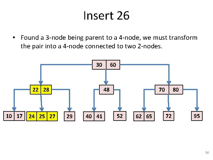
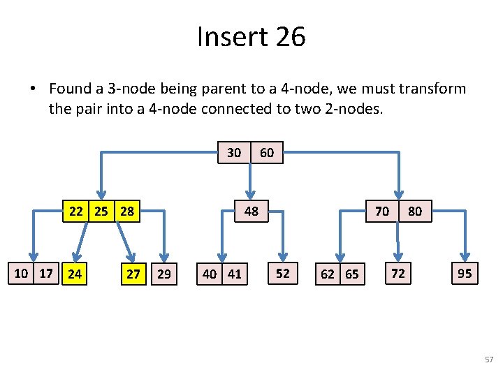
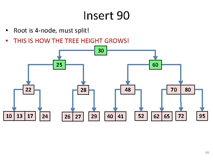
Insertion in 2 -3 -4 Trees • Given our key K: we follow the same path as in search. • On the way we “fix“ all the 4 nodes we meet: – If the parent is a 2 -node, transform the pair into a 3 -node connected to two 2 -nodes. – If the parent is a 3 -node, we transform the pair into a 4 -node connected to two 2 -nodes. – If there is no parent (the root itself is a 4 -node), split it into three 2 nodes (root and children). - This is how the tree height grows. • These transformations: – Are local (they only affect the nodes in question). – Do not affect the overall balance or height of the tree (except for splitting a 4 -node root). • This way, when we get to the bottom of the tree, we know that the node we arrived at is not a 4 -node, and thus it has room to insert the new item. 37

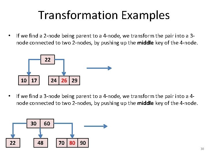
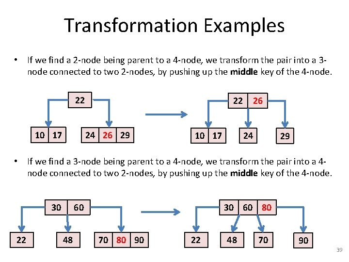
Transformation Examples • If we find a 2 -node being parent to a 4 -node, we transform the pair into a 3 node connected to two 2 -nodes, by pushing up the middle key of the 4 -node. 22 10 17 24 26 29 • If we find a 3 -node being parent to a 4 -node, we transform the pair into a 4 node connected to two 2 -nodes, by pushing up the middle key of the 4 -node. 30 22 60 48 70 80 90 38

Transformation Examples • If we find a 2 -node being parent to a 4 -node, we transform the pair into a 3 node connected to two 2 -nodes, by pushing up the middle key of the 4 -node. 22 10 17 22 24 26 29 26 24 10 17 29 • If we find a 3 -node being parent to a 4 -node, we transform the pair into a 4 node connected to two 2 -nodes, by pushing up the middle key of the 4 -node. 30 22 60 48 30 60 80 70 80 90 22 48 70 90 39

Insertion Examples 40

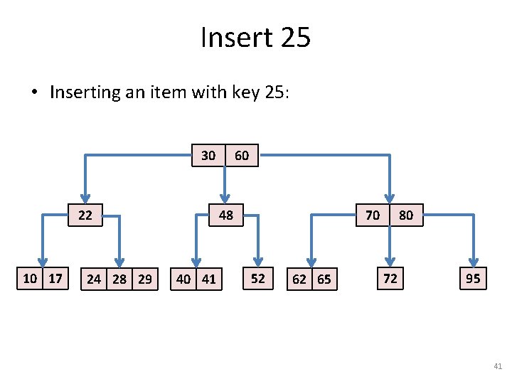
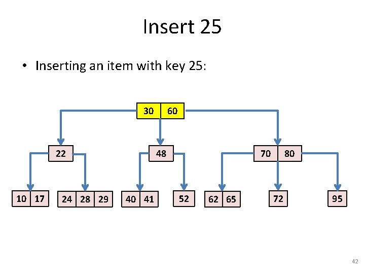
Insert 25 • Inserting an item with key 25: 30 22 10 17 24 28 29 60 48 40 41 70 52 62 65 80 72 95 41

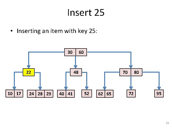
Insert 25 • Inserting an item with key 25: 30 22 10 17 24 28 29 60 48 40 41 70 52 62 65 80 72 95 42

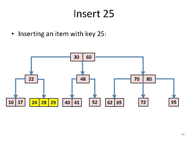
Insert 25 • Inserting an item with key 25: 30 22 10 17 24 28 29 60 48 40 41 70 52 62 65 80 72 95 43

Insert 25 • Inserting an item with key 25: 30 22 10 17 24 28 29 60 48 40 41 70 52 62 65 80 72 95 44

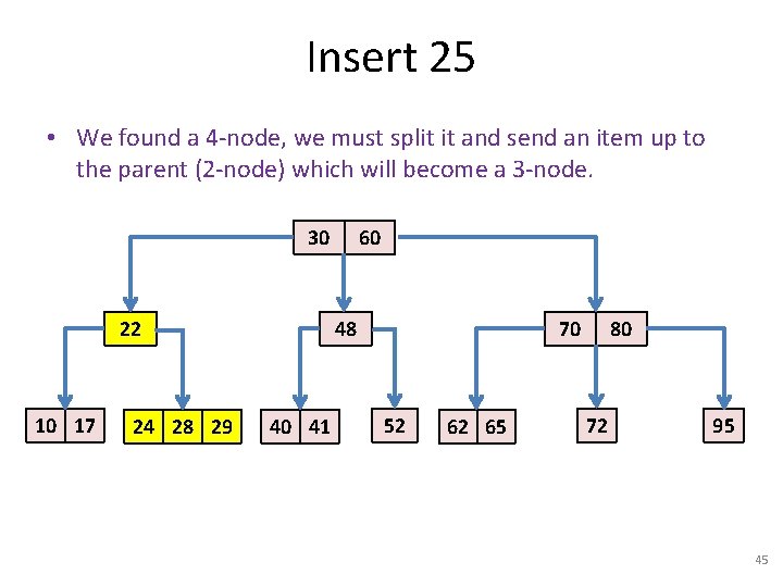
Insert 25 • We found a 4 -node, we must split it and send an item up to the parent (2 -node) which will become a 3 -node. 30 22 10 17 24 28 29 60 48 40 41 70 52 62 65 80 72 95 45

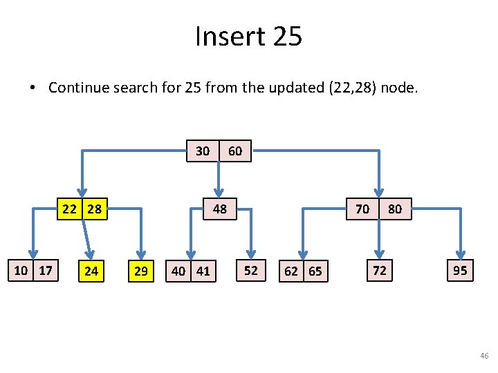
Insert 25 • Continue search for 25 from the updated (22, 28) node. 30 22 28 10 17 24 60 48 29 40 41 70 52 62 65 80 72 95 46

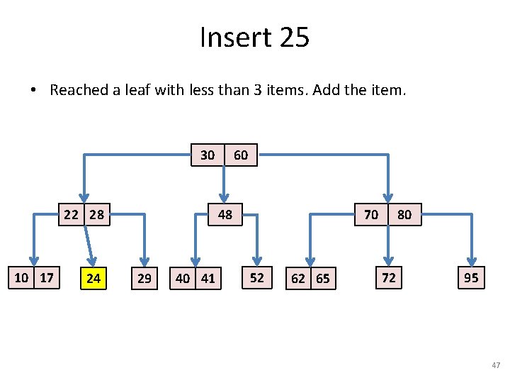
Insert 25 • Reached a leaf with less than 3 items. Add the item. 30 22 28 10 17 24 60 48 29 40 41 70 52 62 65 80 72 95 47

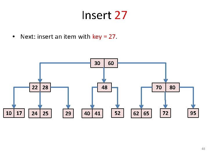
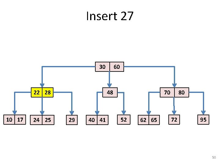
Insert 27 • Next: insert an item with key = 27. 30 22 28 10 17 24 25 60 48 29 40 41 70 52 62 65 80 72 95 48

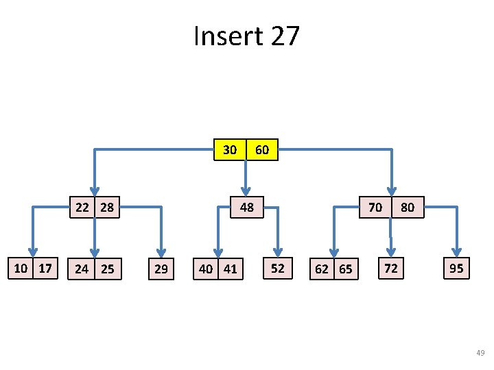
Insert 27 30 22 28 10 17 24 25 60 48 29 40 41 70 52 62 65 80 72 95 49

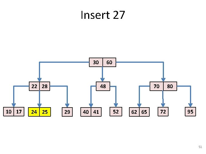
Insert 27 30 22 28 10 17 24 25 60 48 29 40 41 70 52 62 65 80 72 95 50

Insert 27 30 22 28 10 17 24 25 60 48 29 40 41 70 52 62 65 80 72 95 51

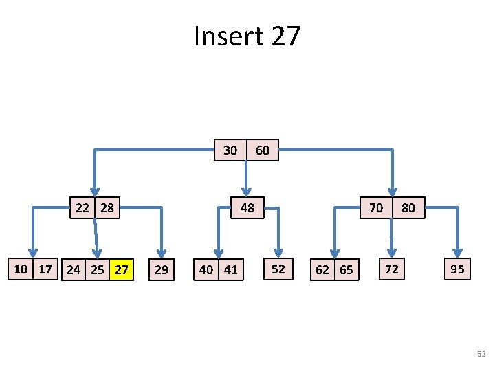
Insert 27 30 22 28 10 17 24 25 27 60 48 29 40 41 70 52 62 65 80 72 95 52

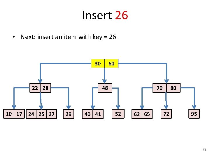
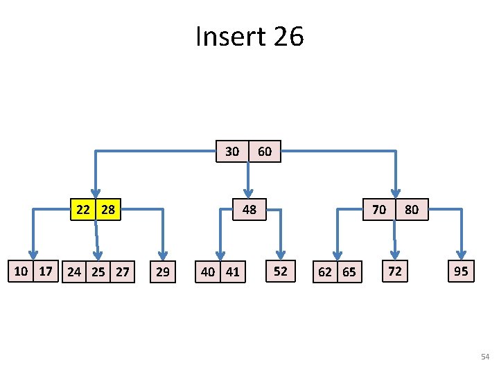
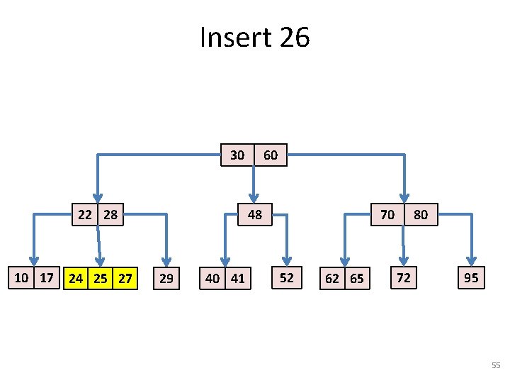
Insert 26 • Next: insert an item with key = 26. 30 22 28 10 17 24 25 27 60 48 29 40 41 70 52 62 65 80 72 95 53

Insert 26 30 22 28 10 17 24 25 27 60 48 29 40 41 70 52 62 65 80 72 95 54

Insert 26 30 22 28 10 17 24 25 27 60 48 29 40 41 70 52 62 65 80 72 95 55

Insert 26 • Found a 3 -node being parent to a 4 -node, we must transform the pair into a 4 -node connected to two 2 -nodes. 30 22 28 10 17 24 25 27 60 48 29 40 41 70 52 62 65 80 72 95 56

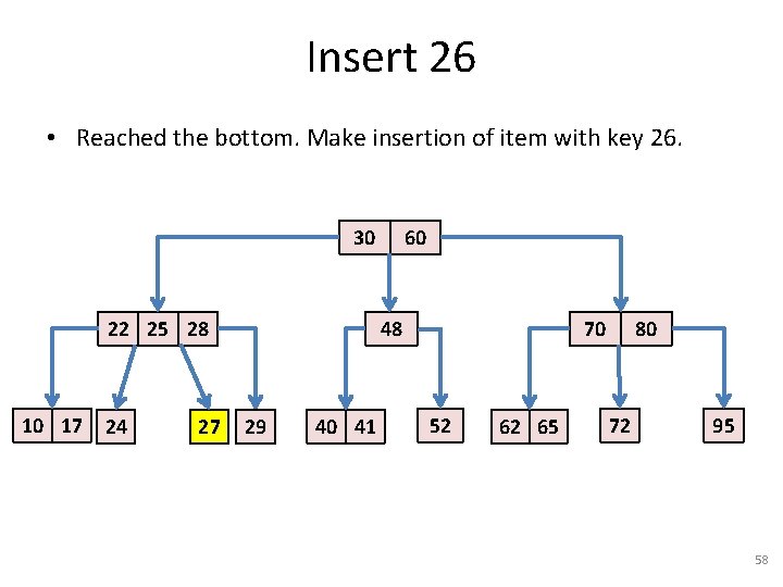
Insert 26 • Found a 3 -node being parent to a 4 -node, we must transform the pair into a 4 -node connected to two 2 -nodes. 30 22 25 28 10 17 24 27 60 48 29 40 41 70 52 62 65 80 72 95 57

Insert 26 • Reached the bottom. Make insertion of item with key 26. 30 22 25 28 10 17 24 27 60 48 29 40 41 70 52 62 65 80 72 95 58

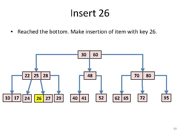
Insert 26 • Reached the bottom. Make insertion of item with key 26. 30 22 25 28 10 17 24 26 27 60 48 29 40 41 70 52 62 65 80 72 95 59

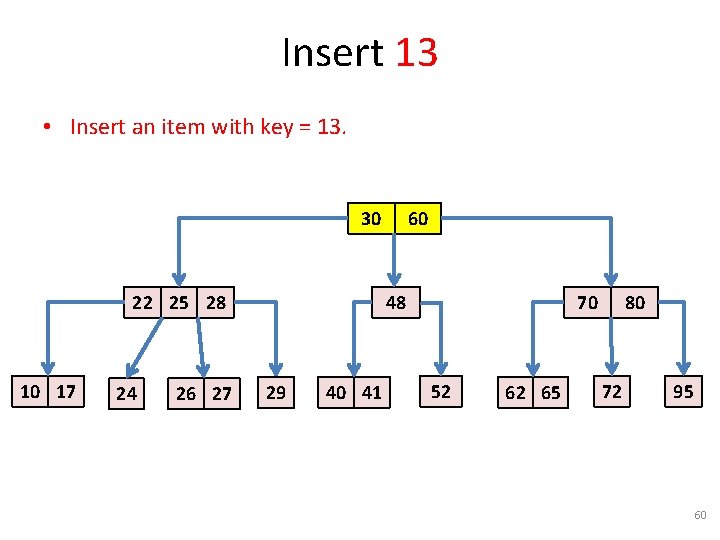
Insert 13 • Insert an item with key = 13. 30 22 25 28 10 17 24 26 27 60 48 29 40 41 70 52 62 65 80 72 95 60

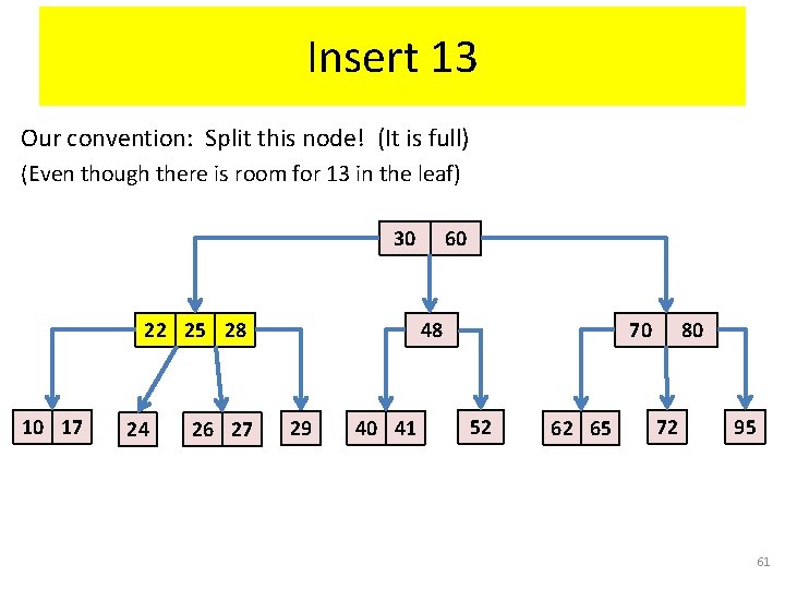
Insert 13 Our convention: Split this node! (It is full) (Even though there is room for 13 in the leaf) 30 22 25 28 10 17 24 26 27 60 48 29 40 41 70 52 62 65 80 72 95 61

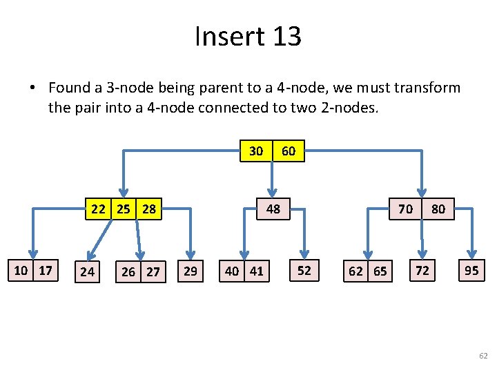
Insert 13 • Found a 3 -node being parent to a 4 -node, we must transform the pair into a 4 -node connected to two 2 -nodes. 30 22 25 28 10 17 24 26 27 60 48 29 40 41 70 52 62 65 80 72 95 62

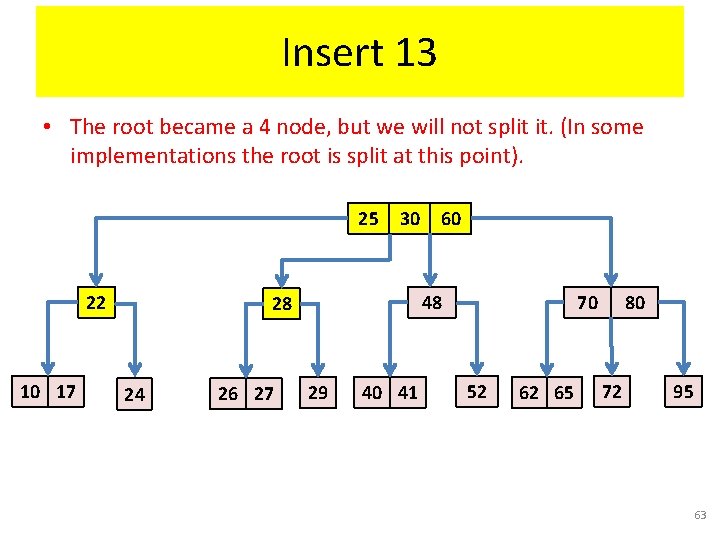
Insert 13 • The root became a 4 node, but we will not split it. (In some implementations the root is split at this point). 25 22 10 17 30 48 28 24 26 27 60 29 40 41 70 52 62 65 80 72 95 63

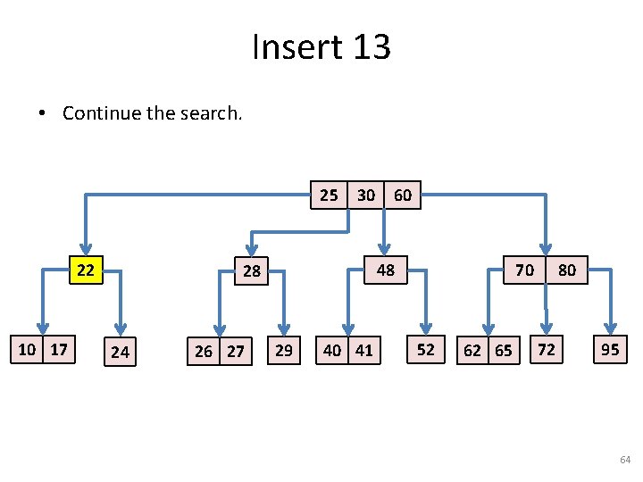
Insert 13 • Continue the search. 25 22 10 17 30 48 28 24 26 27 60 29 40 41 70 52 62 65 80 72 95 64

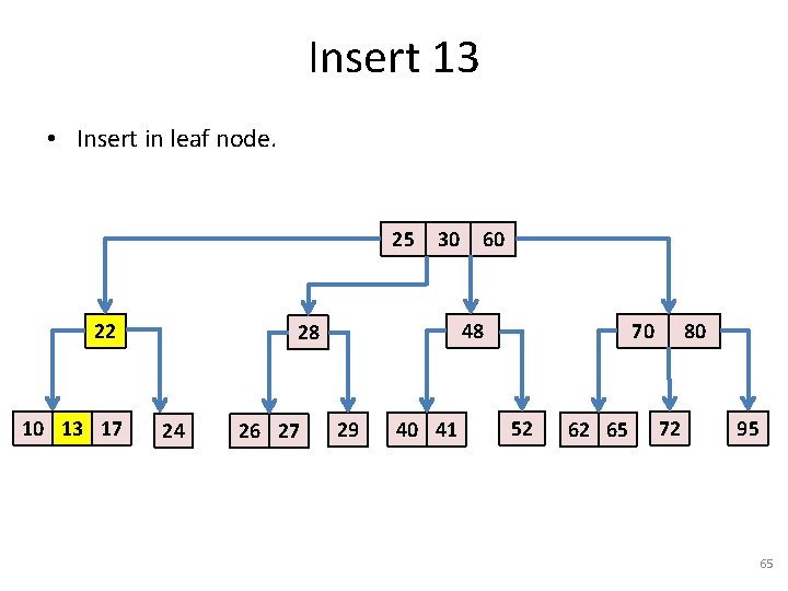
Insert 13 • Insert in leaf node. 25 22 10 13 17 17 30 48 28 24 26 27 60 29 40 41 70 52 62 65 80 72 95 65

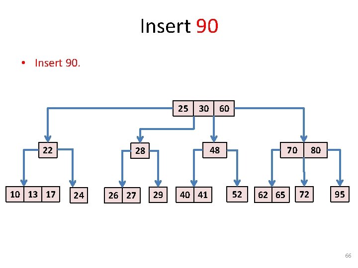
Insert 90 • Insert 90. 25 22 10 13 17 17 30 48 28 24 26 27 60 29 40 41 70 52 62 65 80 72 95 66

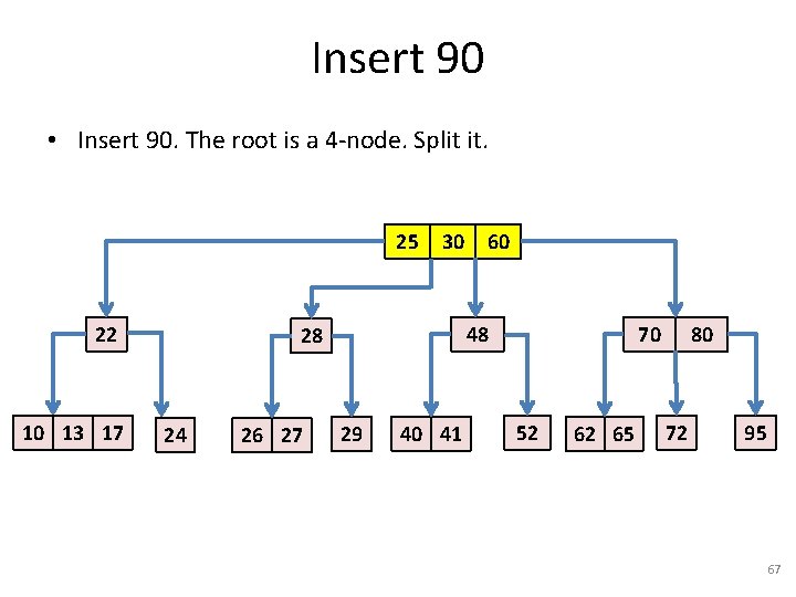
Insert 90 • Insert 90. The root is a 4 -node. Split it. 25 22 10 13 17 17 30 48 28 24 26 27 60 29 40 41 70 52 62 65 80 72 95 67

Insert 90 • Root is 4 -node, must split! • THIS IS HOW THE TREE HEIGHT GROWS! 30 25 22 10 13 17 17 60 48 28 24 26 27 29 40 41 70 52 62 65 80 72 95 68

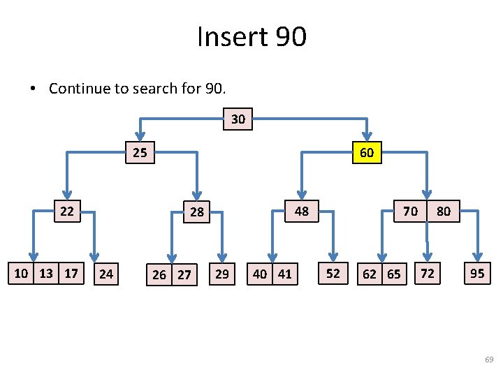
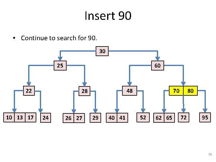
Insert 90 • Continue to search for 90. 30 25 22 10 13 17 17 60 48 28 24 26 27 29 40 41 70 52 62 65 80 72 95 69

Insert 90 • Continue to search for 90. 30 25 22 10 13 17 17 60 48 28 24 26 27 29 40 41 70 52 62 65 80 72 95 70

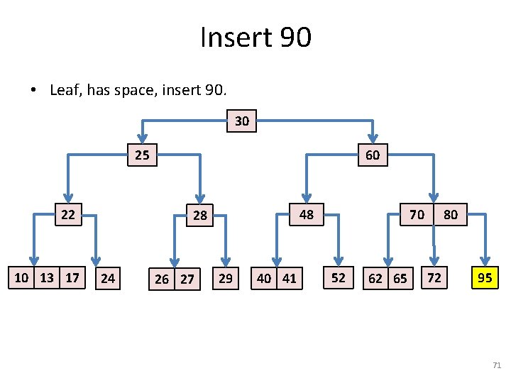
Insert 90 • Leaf, has space, insert 90. 30 25 22 10 13 17 17 60 48 28 24 26 27 29 40 41 70 52 62 65 80 72 95 71

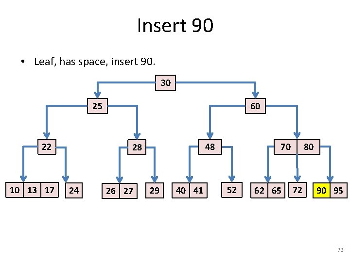
Insert 90 • Leaf, has space, insert 90. 30 25 22 10 13 17 17 60 48 28 24 26 27 29 40 41 70 52 62 65 80 72 90 95 72

REMEMBER our convention • If on your path to insert, you see a 4 node, you split it! • You do that even if there is room in the leaf and you can insert without splitting this node. 73

Deletion in 2 -3 -4 Trees • More complicated. – Sedwick book does not cover it. • Idea: in order to delete item x (with key k) search for k. When find it: – If in a leaf remove it, – Else replace it with the successor of x, y. (y is the item with the first key larger than k. ) Note: y will be in a leaf. • remove y and put it in place of x. • When removing y we have problems as with insert, but now the nodes may not have enough keys (need 2 or 3 keys) => fix nodes that have only one key on the path from root to y. 74

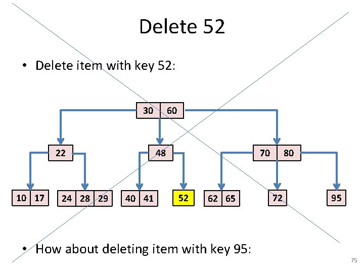
Delete 52 • Delete item with key 52: 30 22 10 17 24 28 29 60 48 40 41 70 52 62 65 • How about deleting item with key 95: 80 72 95 75

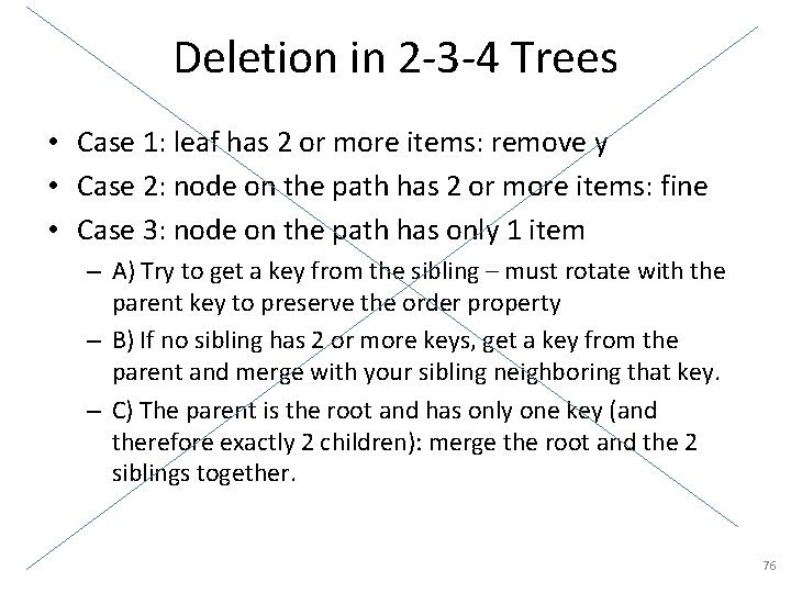
Deletion in 2 -3 -4 Trees • Case 1: leaf has 2 or more items: remove y • Case 2: node on the path has 2 or more items: fine • Case 3: node on the path has only 1 item – A) Try to get a key from the sibling – must rotate with the parent key to preserve the order property – B) If no sibling has 2 or more keys, get a key from the parent and merge with your sibling neighboring that key. – C) The parent is the root and has only one key (and therefore exactly 2 children): merge the root and the 2 siblings together. 76

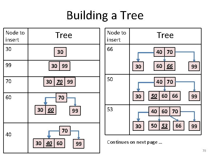
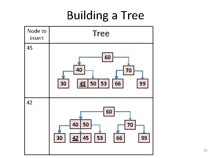
Example: Build a Tree • In an empty tree, insert items given in order: 30, 99, 70, 60, 40, 66, 50, 53, 45, 42 77

Building a Tree Node to insert 30 66 30 99 70 30 70 99 60 40 50 53 99 99 50 60 66 99 40 60 70 30 70 60 66 40 70 30 99 30 40 60 40 70 30 60 Tree Node to insert 50 53 66 99 Continues on next page … 78

Building a Tree Node to insert 45 60 40 30 70 45 50 53 66 99 42 60 40 50 30 42 45 70 53 66 99 79

Self Balancing Binary Trees • • Red-Black trees AVL trees Splay trees …. 80

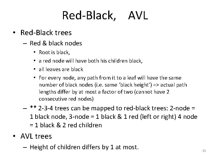
Red-Black, AVL • Red-Black trees – Red & black nodes • • Root is black, a red node will have both his children black, all leaves are black For every node, any path from it to a leaf will have the same number of black nodes (i. e. same ‘black height’) => actual path lengths differ by at most a factor of two (cannot have 2 consecutive red nodes) – ** 2 -3 -4 trees can be mapped to red-black trees: 2 -node = 1 black node, 3 -node = 1 black & 1 red (left or right) 4 node = 1 black & 2 red children • AVL trees – Height of children differs by 1 at most. 81

Splay trees • Splay trees – Self adjusting: the items used more recently (inserted or read/visited) move towards the top. – The tree is not balanced, but performs well because it brings the frequent items to the top. – Splay insertion: the new item is inserted at the root by a rotation that replaces a node with his grandchild. • Search in the tree for the new node. It takes you to a leaf location. Insert new node there and continue with repeated rotations to bring it to the root. This process will reduce the length of that original path to half (because with each rotation, the grandchild node moves two levels up => the path on which these rotations are done, is cut in half). – Can apply the splay operation when searching for an item as well. • See Sedgewick page 545, for this effect. 82