Search Search plays a key role in many

Search • Search plays a key role in many parts of AI. These algorithms provide the conceptual backbone of almost every approach to the systematic exploration of alternatives. • There are four classes of search algorithms, which differ along two dimensions: – First, is the difference between uninformed (also known as blind) search and then informed (also known as heuristic) searches. • Informed searches have access to task-specific information that can be used to make the search process more efficient. – The other difference is between any solution searches and optimal searches. • Optimal searches are looking for the best possible solution while anypath searches will just settle for finding some solution.

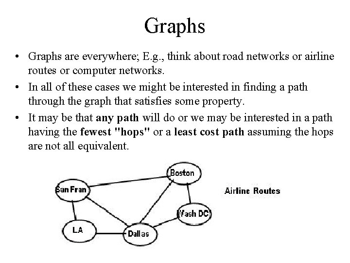
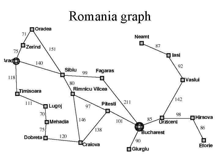
Graphs • Graphs are everywhere; E. g. , think about road networks or airline routes or computer networks. • In all of these cases we might be interested in finding a path through the graph that satisfies some property. • It may be that any path will do or we may be interested in a path having the fewest "hops" or a least cost path assuming the hops are not all equivalent.

Romania graph

Formulating the problem • On holiday in Romania; currently in Arad. • Flight leaves tomorrow from Bucharest. • Formulate goal: – be in Bucharest • Formulate problem: – states: various cities – actions: drive between cities • Find solution: – sequence of cities, e. g. , Arad, Sibiu, Fagaras, Bucharest

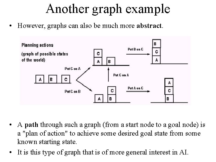
Another graph example • However, graphs can also be much more abstract. • A path through such a graph (from a start node to a goal node) is a "plan of action" to achieve some desired goal state from some known starting state. • It is this type of graph that is of more general interest in AI.

Problem solving • One general approach to problem solving in AI is to reduce the problem to be solved to one of searching a graph. • To use this approach, we must specify what are the states, the actions and the goal test. • A state is supposed to be complete, that is, to represent all the relevant aspects of the problem to be solved. • We are assuming that the actions are deterministic, that is, we know exactly the state after the action is performed.

Goal test • In general, we need a test for the goal, not just one specific goal state. – So, for example, we might be interested in any city in Germany rather than specifically Frankfurt. • Or, when proving a theorem, all we care is about knowing one fact in our current data base of facts. – Any final set of facts that contains the desired fact is a proof.

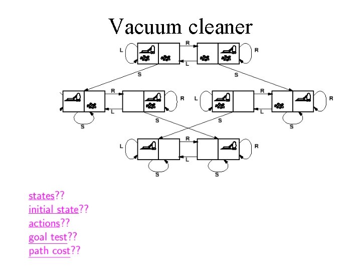
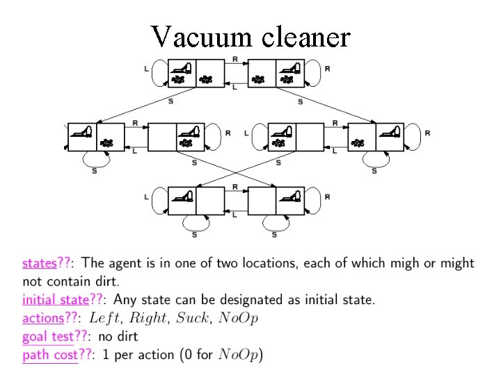
Vacuum cleaner?

Vacuum cleaner

Vacuum cleaner

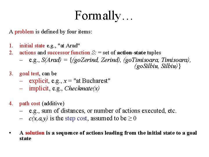
Formally… A problem is defined by four items: 1. 2. initial state e. g. , "at Arad" actions and successor function S: = set of action-state tuples – e. g. , S(Arad) = {(go. Zerind, Zerind), (go. Timisoara, Timisoara), (go. Silbiu, Silbiu)} 3. goal test, can be – explicit, e. g. , x = "at Bucharest" – implicit, e. g. , Checkmate(x) 4. path cost (additive) – e. g. , sum of distances, or number of actions executed, etc. – c(x, a, y) is the step cost, assumed to be ≥ 0 • A solution is a sequence of actions leading from the initial state to a goal state

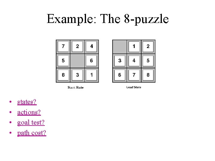
Example: The 8 -puzzle • • states? actions? goal test? path cost?

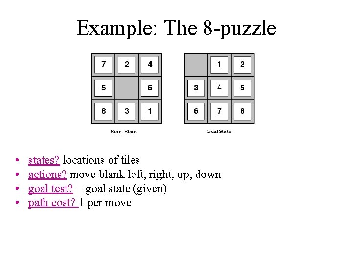
Example: The 8 -puzzle • • states? locations of tiles actions? move blank left, right, up, down goal test? = goal state (given) path cost? 1 per move

Romania graph

Tree search example

Tree search example

Tree search example

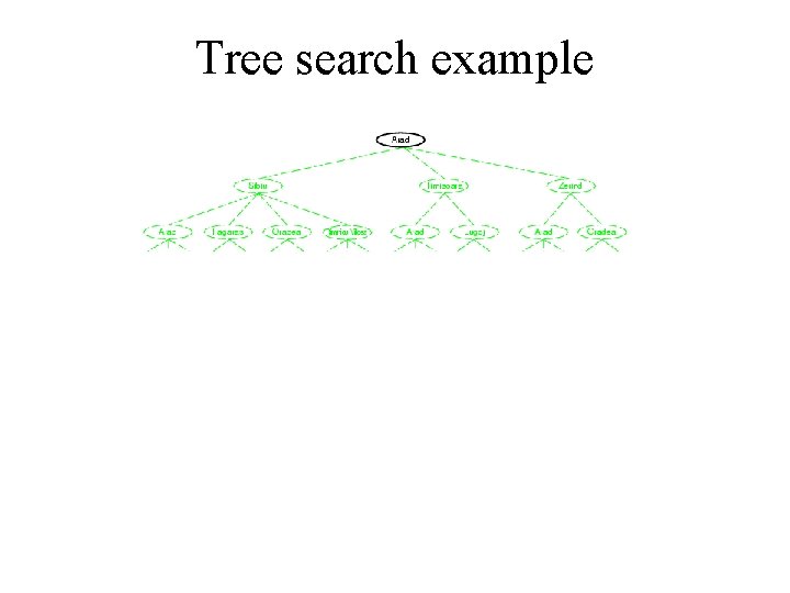
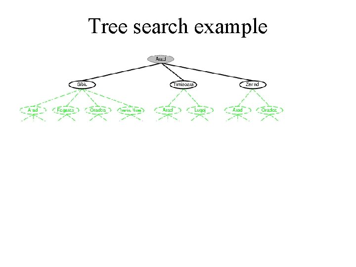
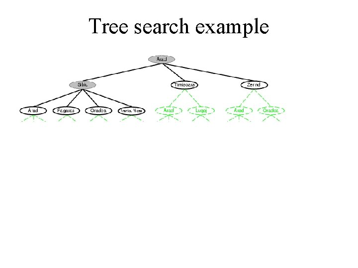
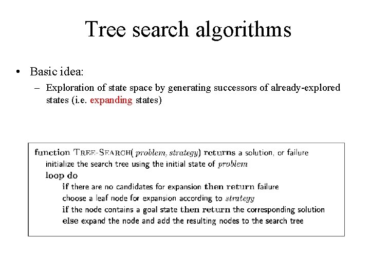
Tree search algorithms • Basic idea: – Exploration of state space by generating successors of already-explored states (i. e. expanding states)

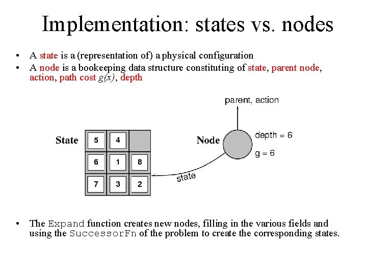
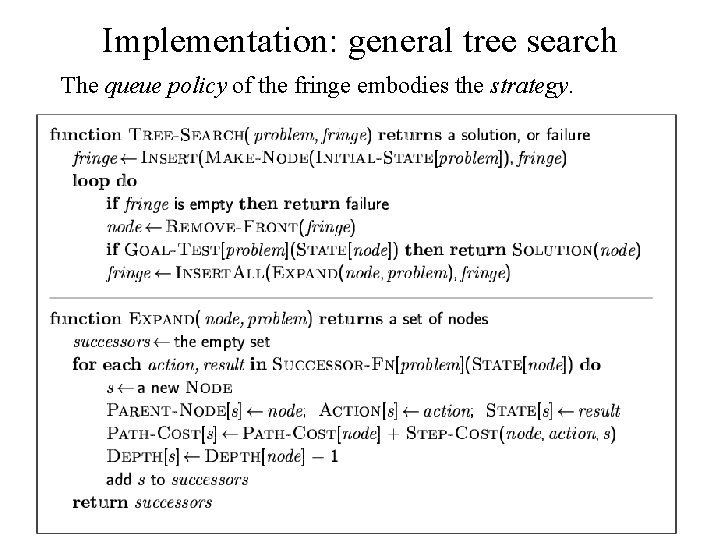
Implementation: states vs. nodes • A state is a (representation of) a physical configuration • A node is a bookeeping data structure constituting of state, parent node, action, path cost g(x), depth • The Expand function creates new nodes, filling in the various fields and using the Successor. Fn of the problem to create the corresponding states.

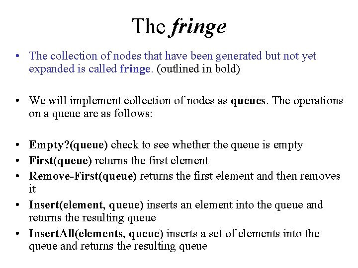
The fringe • The collection of nodes that have been generated but not yet expanded is called fringe. (outlined in bold) • We will implement collection of nodes as queues. The operations on a queue are as follows: • Empty? (queue) check to see whether the queue is empty • First(queue) returns the first element • Remove-First(queue) returns the first element and then removes it • Insert(element, queue) inserts an element into the queue and returns the resulting queue • Insert. All(elements, queue) inserts a set of elements into the queue and returns the resulting queue

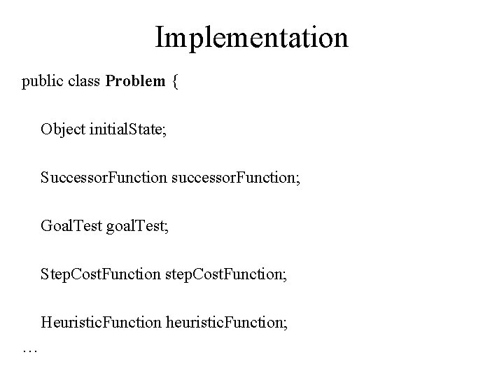
Implementation public class Problem { Object initial. State; Successor. Function successor. Function; Goal. Test goal. Test; Step. Cost. Function step. Cost. Function; Heuristic. Function heuristic. Function; …

Some pseudocode interpretations Successor-Fn[problem](State[node]) is in fact: problem. Successor-Fn(node. State) or problem. get. Successor. Function(). get. Successors( node. get. State() );

Implementation: general tree search The queue policy of the fringe embodies the strategy.

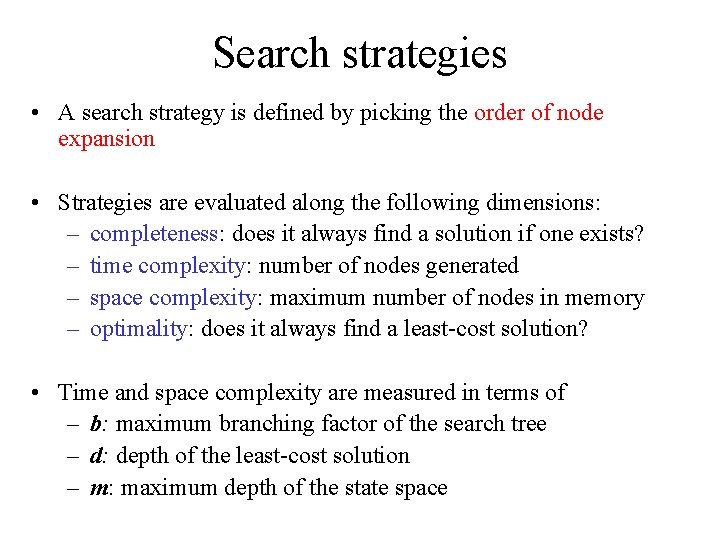
Search strategies • A search strategy is defined by picking the order of node expansion • Strategies are evaluated along the following dimensions: – completeness: does it always find a solution if one exists? – time complexity: number of nodes generated – space complexity: maximum number of nodes in memory – optimality: does it always find a least-cost solution? • Time and space complexity are measured in terms of – b: maximum branching factor of the search tree – d: depth of the least-cost solution – m: maximum depth of the state space

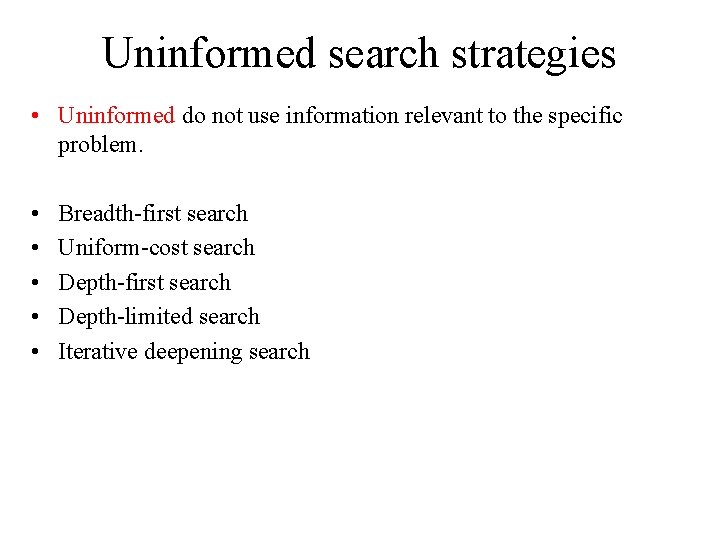
Uninformed search strategies • Uninformed do not use information relevant to the specific problem. • • • Breadth-first search Uniform-cost search Depth-first search Depth-limited search Iterative deepening search

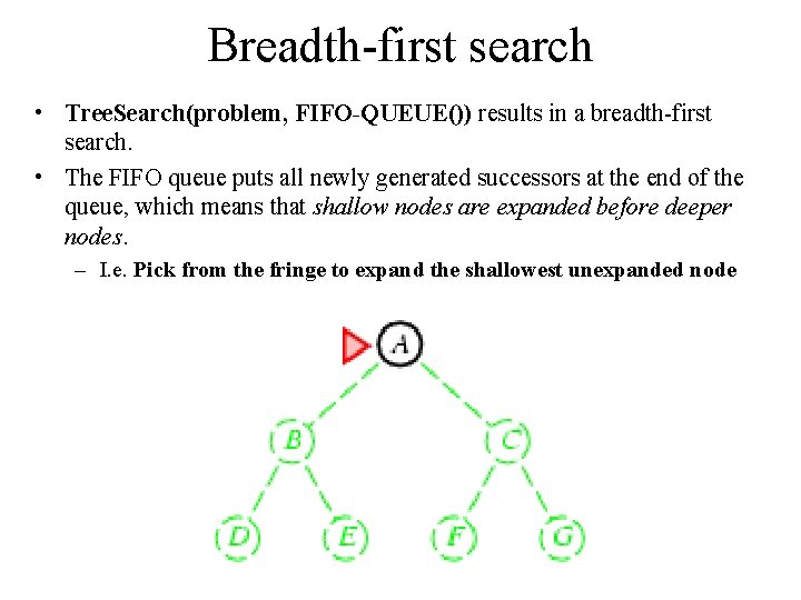
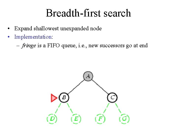
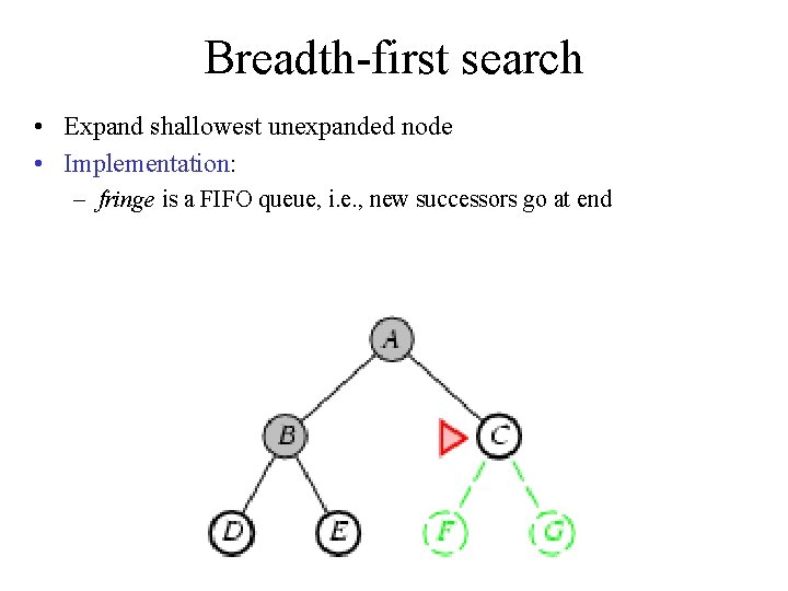
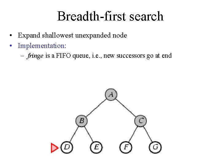
Breadth-first search • Tree. Search(problem, FIFO-QUEUE()) results in a breadth-first search. • The FIFO queue puts all newly generated successors at the end of the queue, which means that shallow nodes are expanded before deeper nodes. – I. e. Pick from the fringe to expand the shallowest unexpanded node

Breadth-first search • Expand shallowest unexpanded node • Implementation: – fringe is a FIFO queue, i. e. , new successors go at end

Breadth-first search • Expand shallowest unexpanded node • Implementation: – fringe is a FIFO queue, i. e. , new successors go at end

Breadth-first search • Expand shallowest unexpanded node • Implementation: – fringe is a FIFO queue, i. e. , new successors go at end

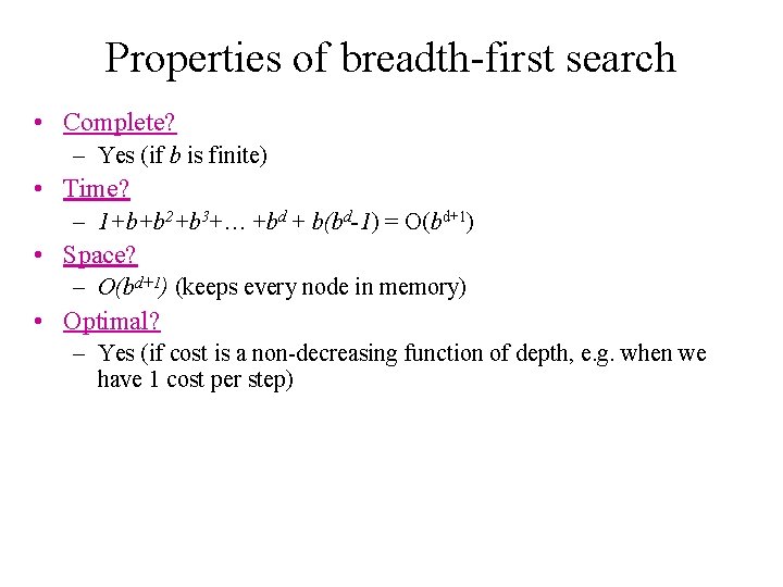
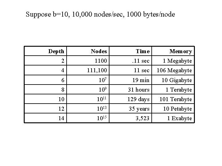
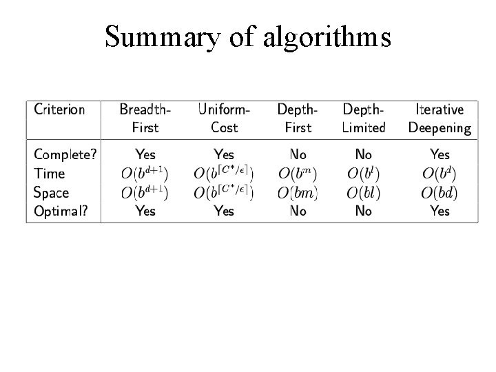
Properties of breadth-first search • Complete? – Yes (if b is finite) • Time? – 1+b+b 2+b 3+… +bd + b(bd-1) = O(bd+1) • Space? – O(bd+1) (keeps every node in memory) • Optimal? – Yes (if cost is a non-decreasing function of depth, e. g. when we have 1 cost per step)

Suppose b=10, 000 nodes/sec, 1000 bytes/node Depth Nodes Time Memory 2 1100 . 11 sec 1 Megabyte 4 111, 100 11 sec 106 Megabyte 6 107 19 min 10 Gigabyte 8 109 31 hours 1 Terabyte 10 1011 129 days 101 Terabyte 12 1013 35 years 10 Petabyte 14 1015 3, 523 1 Exabyte

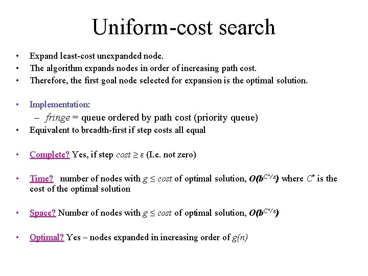
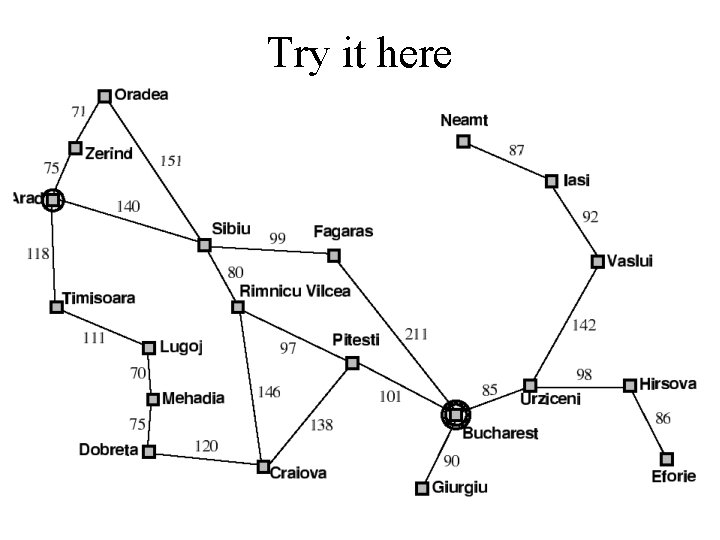
Uniform-cost search • • • Expand least-cost unexpanded node. The algorithm expands nodes in order of increasing path cost. Therefore, the first goal node selected for expansion is the optimal solution. • Implementation: – fringe = queue ordered by path cost (priority queue) • Equivalent to breadth-first if step costs all equal • Complete? Yes, if step cost ≥ ε (I. e. not zero) • Time? number of nodes with g ≤ cost of optimal solution, O(b. C*/ ε) where C* is the cost of the optimal solution • Space? Number of nodes with g ≤ cost of optimal solution, O(b. C*/ ε) • Optimal? Yes – nodes expanded in increasing order of g(n)

Try it here

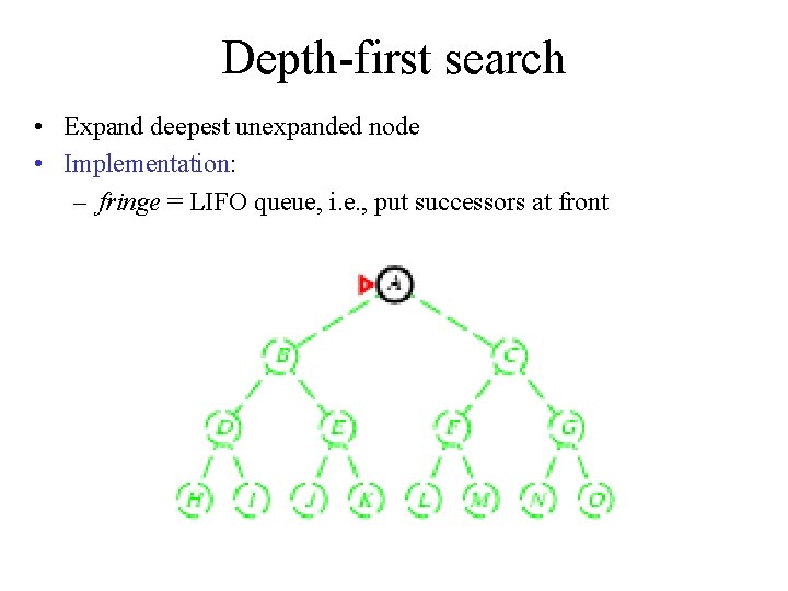
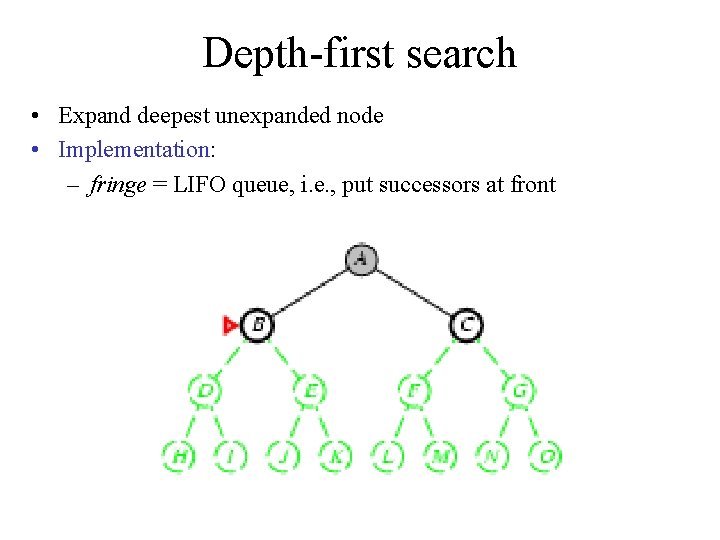
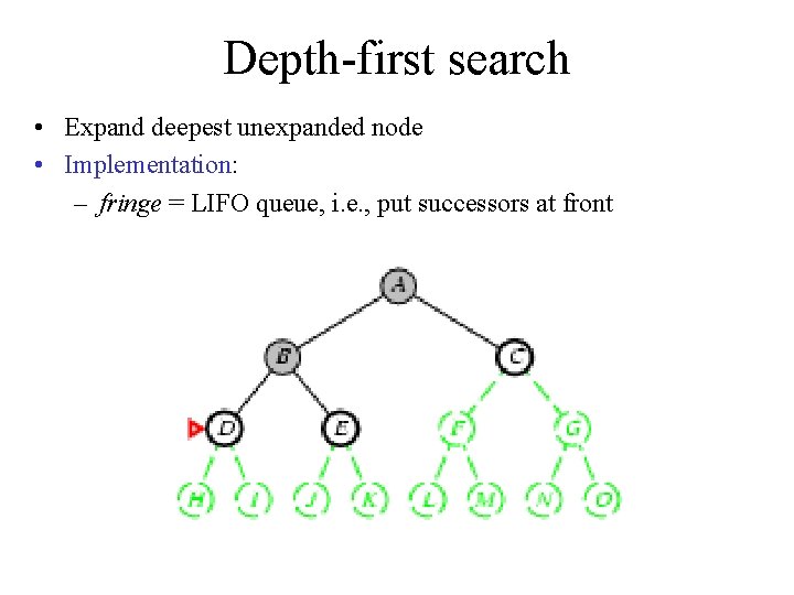
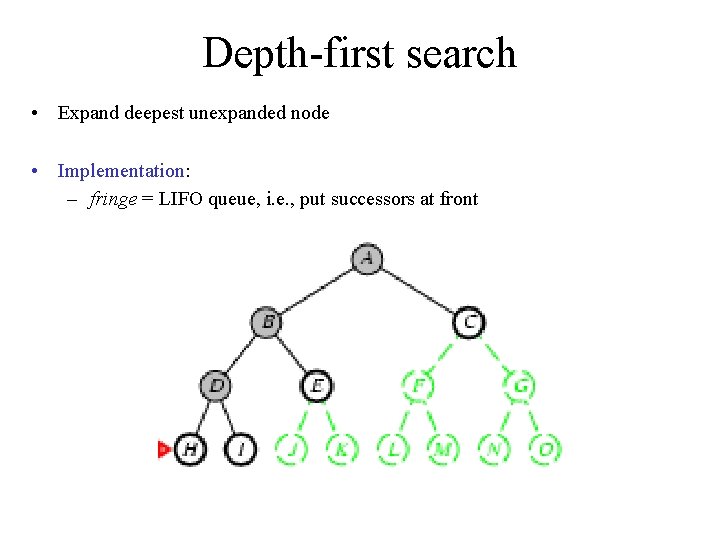
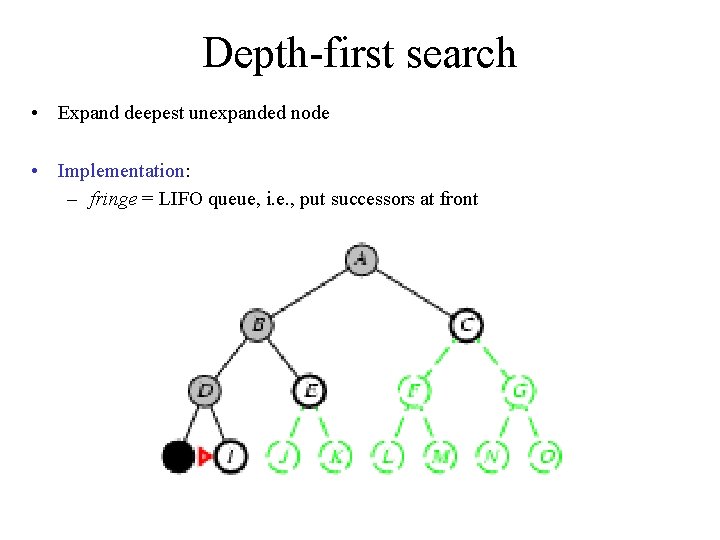
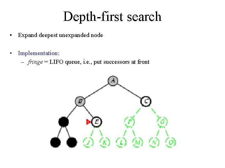
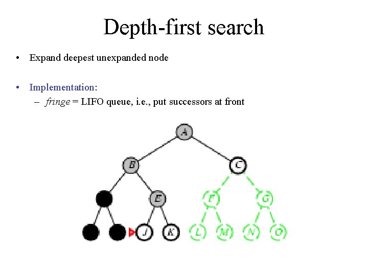
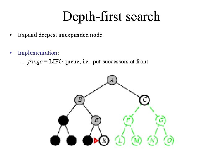
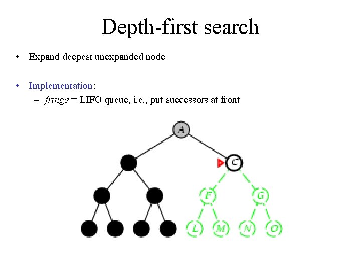
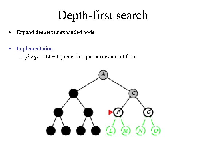
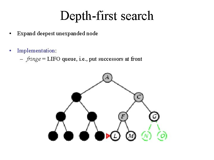
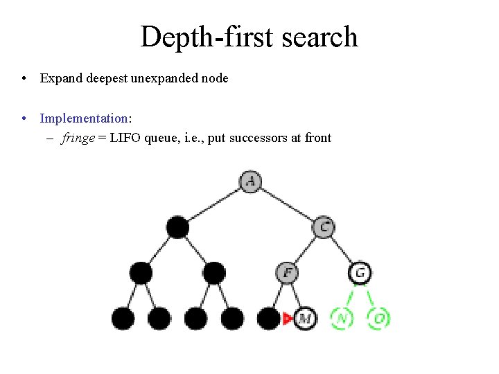
Depth-first search • Expand deepest unexpanded node • Implementation: – fringe = LIFO queue, i. e. , put successors at front

Depth-first search • Expand deepest unexpanded node • Implementation: – fringe = LIFO queue, i. e. , put successors at front

Depth-first search • Expand deepest unexpanded node • Implementation: – fringe = LIFO queue, i. e. , put successors at front

Depth-first search • Expand deepest unexpanded node • Implementation: – fringe = LIFO queue, i. e. , put successors at front

Depth-first search • Expand deepest unexpanded node • Implementation: – fringe = LIFO queue, i. e. , put successors at front

Depth-first search • Expand deepest unexpanded node • Implementation: – fringe = LIFO queue, i. e. , put successors at front

Depth-first search • Expand deepest unexpanded node • Implementation: – fringe = LIFO queue, i. e. , put successors at front

Depth-first search • Expand deepest unexpanded node • Implementation: – fringe = LIFO queue, i. e. , put successors at front

Depth-first search • Expand deepest unexpanded node • Implementation: – fringe = LIFO queue, i. e. , put successors at front

Depth-first search • Expand deepest unexpanded node • Implementation: – fringe = LIFO queue, i. e. , put successors at front

Depth-first search • Expand deepest unexpanded node • Implementation: – fringe = LIFO queue, i. e. , put successors at front

Depth-first search • Expand deepest unexpanded node • Implementation: – fringe = LIFO queue, i. e. , put successors at front

Properties of depth-first search • Complete? No: fails in infinite-depth spaces, spaces with loops – Modify to avoid repeated states along path complete in finite spaces • Time? O(bm): terrible if m is much larger than d – but if solutions are dense, may be much faster than breadth-first • Space? O(bm), i. e. , linear space! • Optimal? No

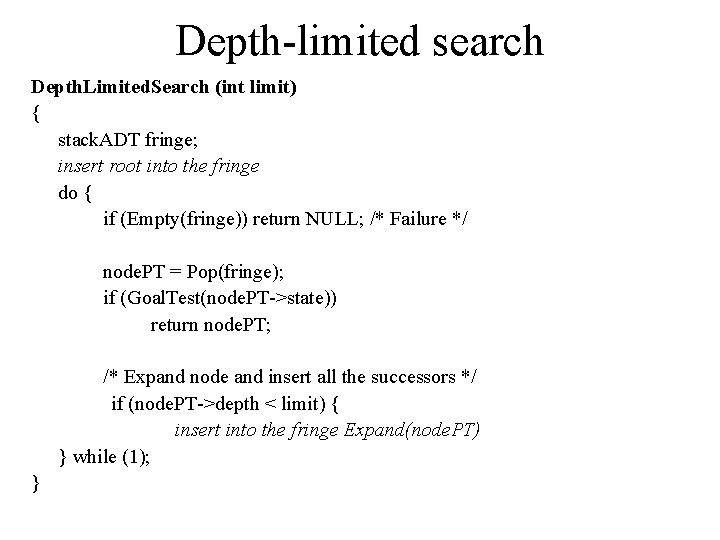
Depth-limited search Depth. Limited. Search (int limit) { stack. ADT fringe; insert root into the fringe do { if (Empty(fringe)) return NULL; /* Failure */ node. PT = Pop(fringe); if (Goal. Test(node. PT->state)) return node. PT; /* Expand node and insert all the successors */ if (node. PT->depth < limit) { insert into the fringe Expand(node. PT) } while (1); }

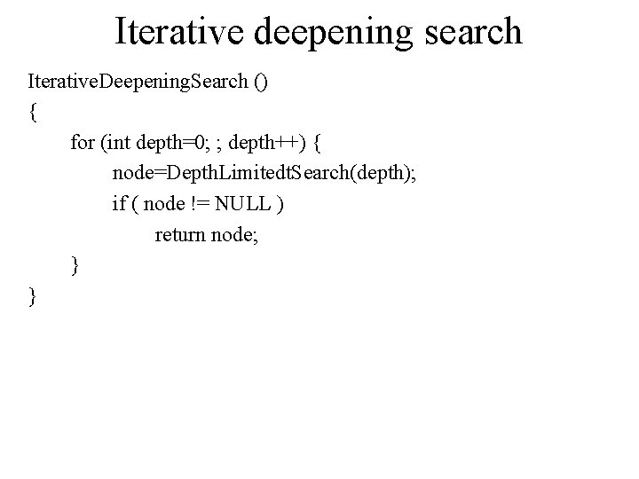
Iterative deepening search Iterative. Deepening. Search () { for (int depth=0; ; depth++) { node=Depth. Limitedt. Search(depth); if ( node != NULL ) return node; } }

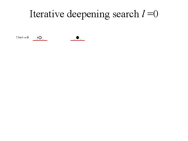
Iterative deepening search l =0

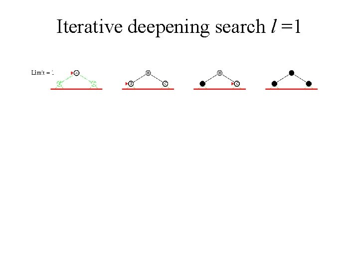
Iterative deepening search l =1

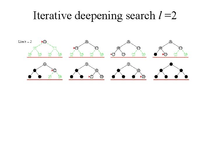
Iterative deepening search l =2

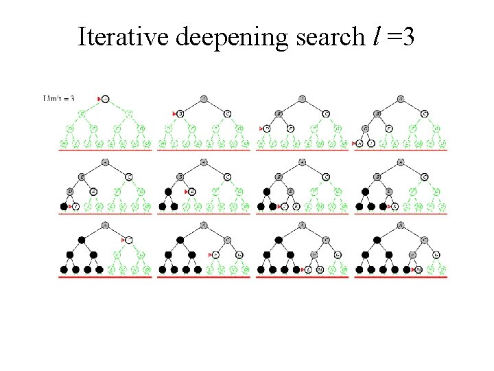
Iterative deepening search l =3

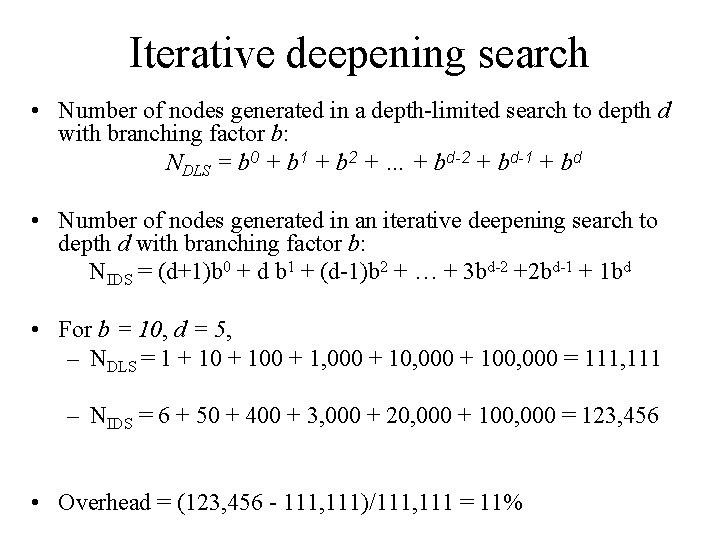
Iterative deepening search • Number of nodes generated in a depth-limited search to depth d with branching factor b: NDLS = b 0 + b 1 + b 2 + … + bd-2 + bd-1 + bd • Number of nodes generated in an iterative deepening search to depth d with branching factor b: NIDS = (d+1)b 0 + d b 1 + (d-1)b 2 + … + 3 bd-2 +2 bd-1 + 1 bd • For b = 10, d = 5, – NDLS = 1 + 100 + 1, 000 + 100, 000 = 111, 111 – NIDS = 6 + 50 + 400 + 3, 000 + 20, 000 + 100, 000 = 123, 456 • Overhead = (123, 456 - 111, 111)/111, 111 = 11%

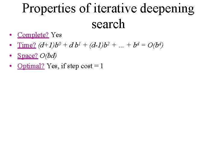
• • Properties of iterative deepening search Complete? Yes Time? (d+1)b 0 + d b 1 + (d-1)b 2 + … + bd = O(bd) Space? O(bd) Optimal? Yes, if step cost = 1

Summary of algorithms

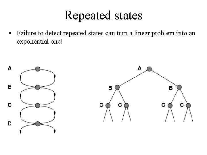
Repeated states • Failure to detect repeated states can turn a linear problem into an exponential one!

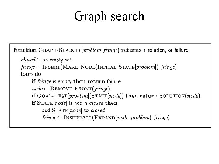
Graph search

Class problem • You have three jugs, measuring 12 gallons, 8 gallons, and 3 gallons, and a water faucet. • You can fill the jugs up, or empty them out from one another or onto the ground. • You need to measure out exactly one gallon.