Search Engines Information Retrieval in Practice All slides

Search Engines Information Retrieval in Practice All slides ©Addison Wesley, 2008

Classification and Clustering • Classification and clustering are classical pattern recognition / machine learning problems • Classification – Asks “what class does this item belong to? ” – Supervised learning task • Clustering – Asks “how can I group this set of items? ” – Unsupervised learning task • Items can be documents, queries, emails, entities, images, etc. • Useful for a wide variety of search engine tasks

Classification • Classification is the task of automatically applying labels to items • Useful for many search-related tasks – Spam detection – Sentiment classification – Online advertising • Two common approaches – Probabilistic – Geometric

How to Classify? • How do humans classify items? • For example, suppose you had to classify the “healthiness” of a food – Identify set of features indicative of health • fat, cholesterol, sugar, sodium, etc. – Extract features from foods • Read nutritional facts, chemical analysis, etc. – Combine evidence from the features into a hypothesis • Add health features together to get “healthiness factor” – Finally, classify the item based on the evidence • If “healthiness factor” is above a certain value, then deem it healthy

Ontologies • Ontology is a labeling or categorization scheme • Examples – Binary (spam, not spam) – Multi-valued (red, green, blue) – Hierarchical (news/local/sports) • Different classification tasks require different ontologies

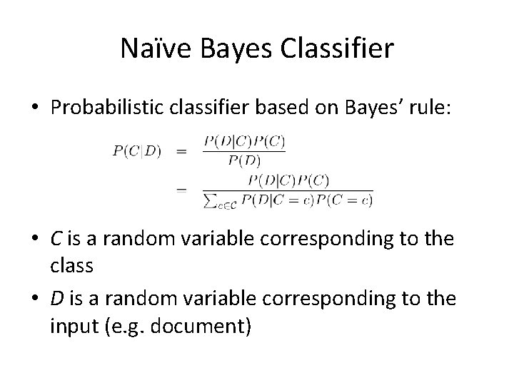
Naïve Bayes Classifier • Probabilistic classifier based on Bayes’ rule: • C is a random variable corresponding to the class • D is a random variable corresponding to the input (e. g. document)

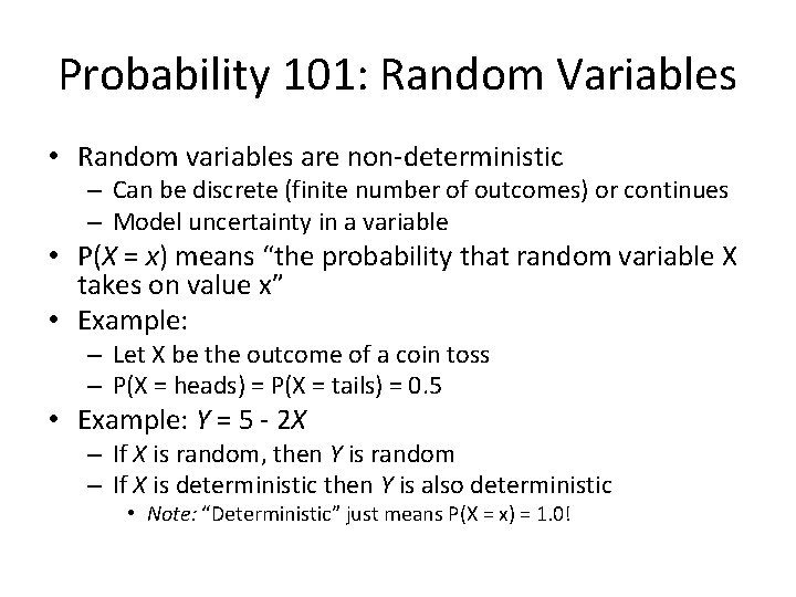
Probability 101: Random Variables • Random variables are non-deterministic – Can be discrete (finite number of outcomes) or continues – Model uncertainty in a variable • P(X = x) means “the probability that random variable X takes on value x” • Example: – Let X be the outcome of a coin toss – P(X = heads) = P(X = tails) = 0. 5 • Example: Y = 5 - 2 X – If X is random, then Y is random – If X is deterministic then Y is also deterministic • Note: “Deterministic” just means P(X = x) = 1. 0!

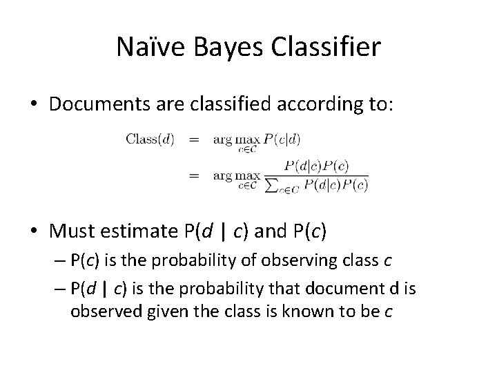
Naïve Bayes Classifier • Documents are classified according to: • Must estimate P(d | c) and P(c) – P(c) is the probability of observing class c – P(d | c) is the probability that document d is observed given the class is known to be c

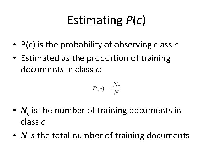
Estimating P(c) • P(c) is the probability of observing class c • Estimated as the proportion of training documents in class c: • Nc is the number of training documents in class c • N is the total number of training documents

Estimating P(d | c) • P(d | c) is the probability that document d is observed given the class is known to be c • Estimate depends on the event space used to represent the documents • What is an event space? – The set of all possible outcomes for a given random variable – For a coin toss random variable the event space is S = {heads, tails}

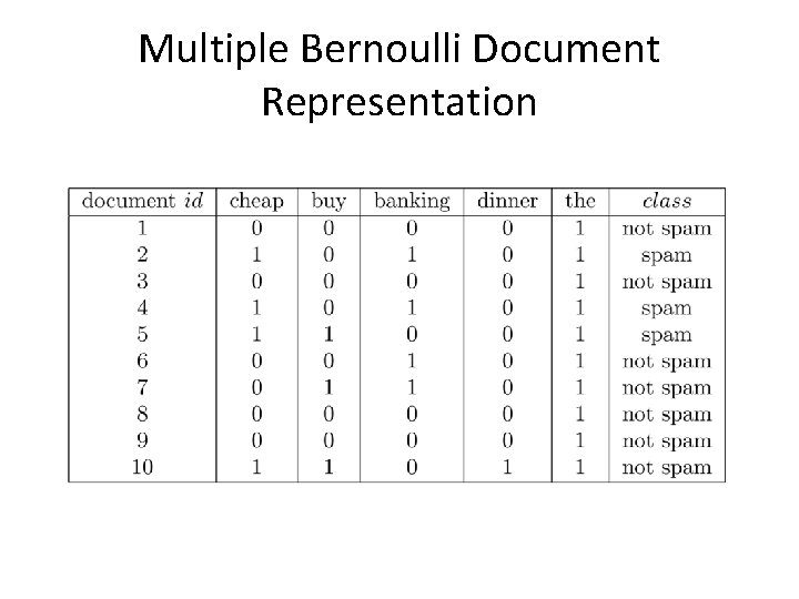
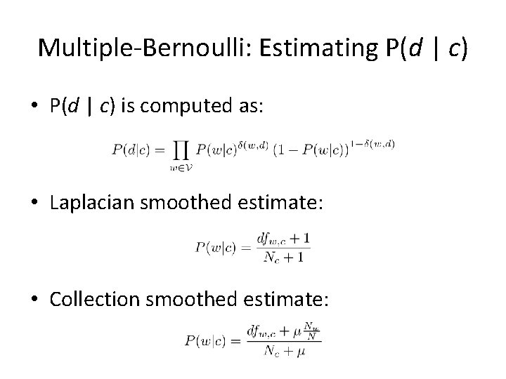
Multiple Bernoulli Event Space • Documents are represented as binary vectors – One entry for every word in the vocabulary – Entry i = 1 if word i occurs in the document and is 0 otherwise • Multiple Bernoulli distribution is a natural way to model distributions over binary vectors • Same event space as used in the classical probabilistic retrieval model

Multiple Bernoulli Document Representation

Multiple-Bernoulli: Estimating P(d | c) • P(d | c) is computed as: • Laplacian smoothed estimate: • Collection smoothed estimate:

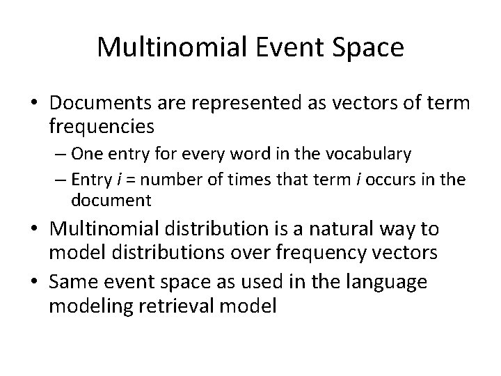
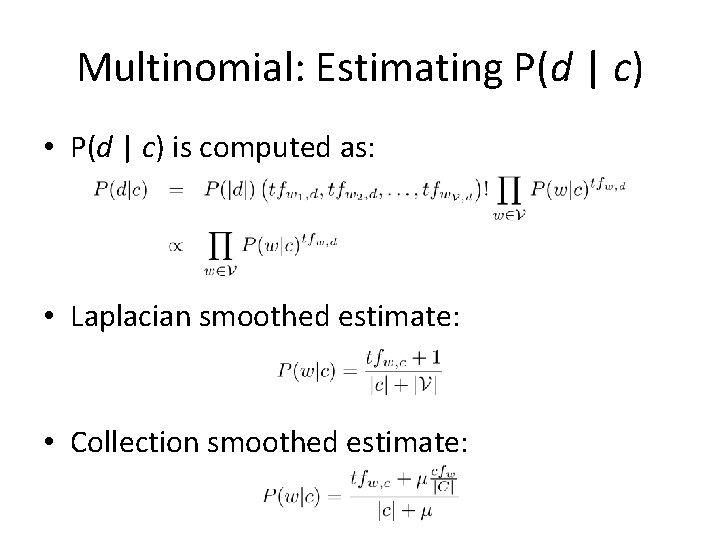
Multinomial Event Space • Documents are represented as vectors of term frequencies – One entry for every word in the vocabulary – Entry i = number of times that term i occurs in the document • Multinomial distribution is a natural way to model distributions over frequency vectors • Same event space as used in the language modeling retrieval model

Multinomial Document Representation

Multinomial: Estimating P(d | c) • P(d | c) is computed as: • Laplacian smoothed estimate: • Collection smoothed estimate:

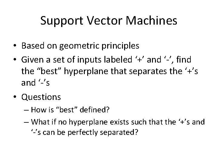
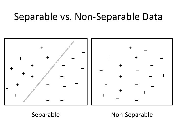
Support Vector Machines • Based on geometric principles • Given a set of inputs labeled ‘+’ and ‘-’, find the “best” hyperplane that separates the ‘+’s and ‘-’s • Questions – How is “best” defined? – What if no hyperplane exists such that the ‘+’s and ‘-’s can be perfectly separated?

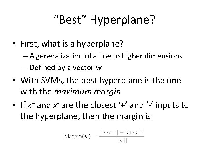
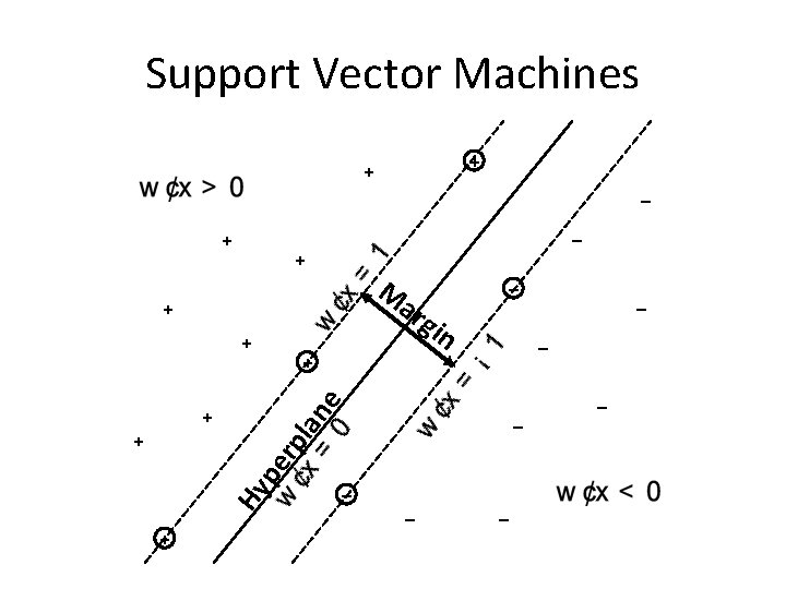
“Best” Hyperplane? • First, what is a hyperplane? – A generalization of a line to higher dimensions – Defined by a vector w • With SVMs, the best hyperplane is the one with the maximum margin • If x+ and x- are the closest ‘+’ and ‘-’ inputs to the hyperplane, then the margin is:

Support Vector Machines + + – + M ar + + ne – pe r – – + Hy + gin pla + + – – –

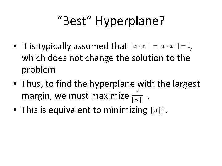
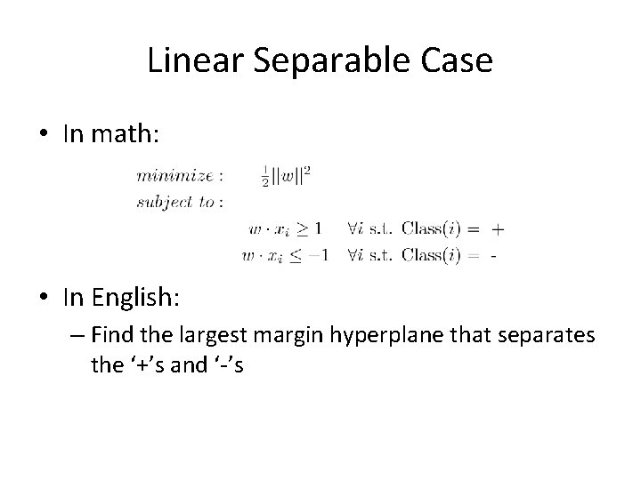
“Best” Hyperplane? • It is typically assumed that , which does not change the solution to the problem • Thus, to find the hyperplane with the largest margin, we must maximize. • This is equivalent to minimizing.

Separable vs. Non-Separable Data + + + + – + – – – Separable – – + + + – + – – Non-Separable +

Linear Separable Case • In math: • In English: – Find the largest margin hyperplane that separates the ‘+’s and ‘-’s

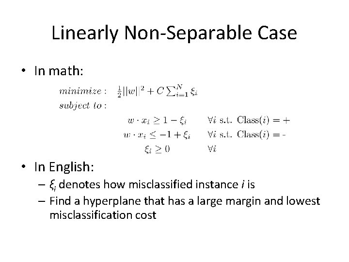
Linearly Non-Separable Case • In math: • In English: – ξi denotes how misclassified instance i is – Find a hyperplane that has a large margin and lowest misclassification cost

The Kernel Trick • Linearly non-separable data may become linearly separable if transformed, or mapped, to a higher dimension space • Computing vector math (i. e. , dot products) in very high dimensional space is costly • The kernel trick allows very high dimensional dot products to be computed efficiently • Allows inputs to be implicitly mapped to high (possibly infinite) dimensional space with little computational overhead

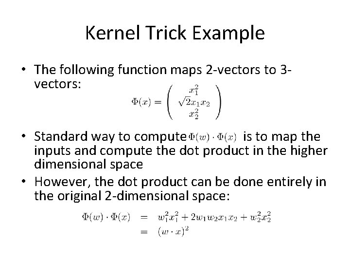
Kernel Trick Example • The following function maps 2 -vectors to 3 vectors: • Standard way to compute is to map the inputs and compute the dot product in the higher dimensional space • However, the dot product can be done entirely in the original 2 -dimensional space:

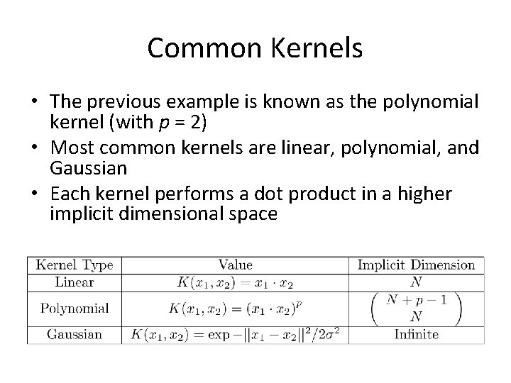
Common Kernels • The previous example is known as the polynomial kernel (with p = 2) • Most common kernels are linear, polynomial, and Gaussian • Each kernel performs a dot product in a higher implicit dimensional space

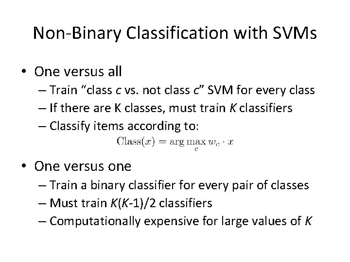
Non-Binary Classification with SVMs • One versus all – Train “class c vs. not class c” SVM for every class – If there are K classes, must train K classifiers – Classify items according to: • One versus one – Train a binary classifier for every pair of classes – Must train K(K-1)/2 classifiers – Computationally expensive for large values of K

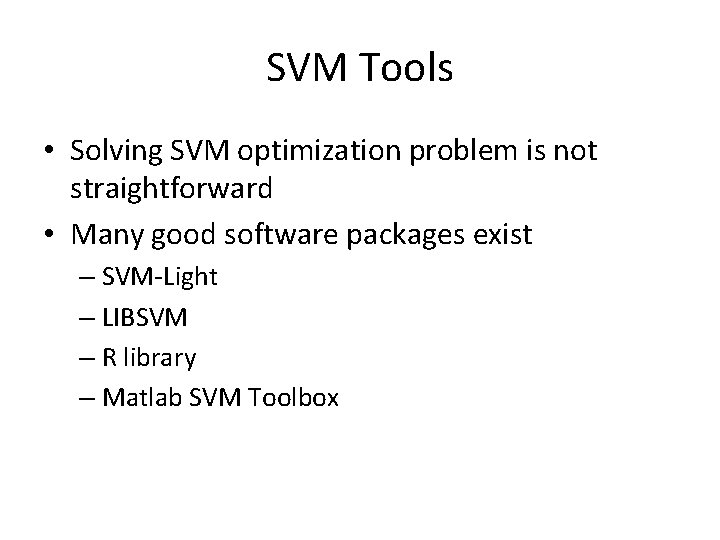
SVM Tools • Solving SVM optimization problem is not straightforward • Many good software packages exist – SVM-Light – LIBSVM – R library – Matlab SVM Toolbox

Evaluating Classifiers • Common classification metrics – Accuracy (precision at rank 1) – Precision – Recall – F-measure – ROC curve analysis • Differences from IR metrics – “Relevant” replaced with “classified correctly” – Microaveraging more commonly used

Classes of Classifiers • Types of classifiers – Generative (Naïve-Bayes) – Discriminative (SVMs) – Non-parametric (nearest neighbor) • Types of learning – Supervised (Naïve-Bayes, SVMs) – Semi-supervised (Rocchio, relevance models) – Unsupervised (clustering)

Generative vs. Discriminative • Generative models – Assumes documents and classes are drawn from joint distribution P(d, c) – Typically P(d, c) decomposed to P(d | c) P(c) – Effectiveness depends on how P(d, c) is modeled – Typically more effective when little training data exists • Discriminative models – Directly model class assignment problem – Do not model document “generation” – Effectiveness depends on amount and quality of training data

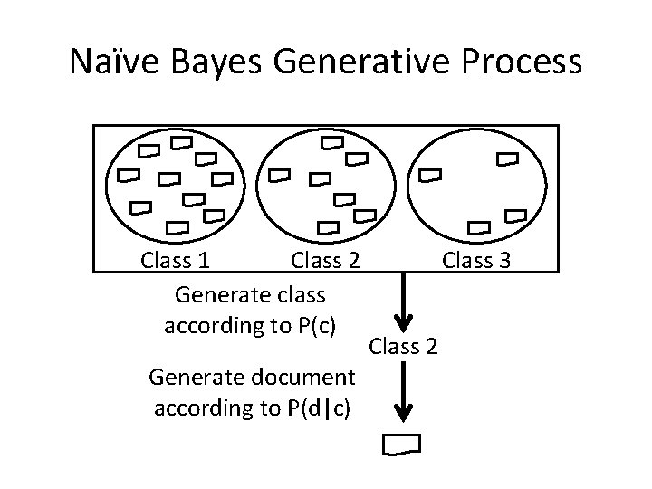
Naïve Bayes Generative Process Class 1 Class 2 Generate class according to P(c) Generate document according to P(d|c) Class 3 Class 2

Feature Selection • Document classifiers can have a very large number of features – Not all features are useful – Excessive features can increase computational cost of training and testing • Feature selection methods reduce the number of features by choosing the most useful features

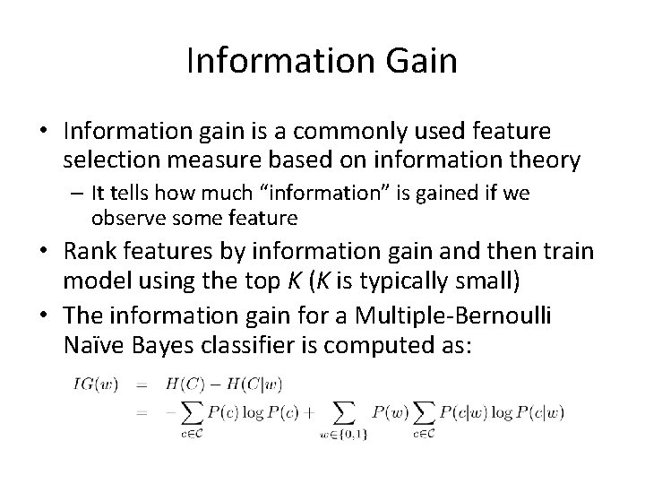
Information Gain • Information gain is a commonly used feature selection measure based on information theory – It tells how much “information” is gained if we observe some feature • Rank features by information gain and then train model using the top K (K is typically small) • The information gain for a Multiple-Bernoulli Naïve Bayes classifier is computed as:

Classification Applications • Classification is widely used to enhance search engines • Example applications – Spam detection – Sentiment classification – Semantic classification of advertisements – Many others not covered here!

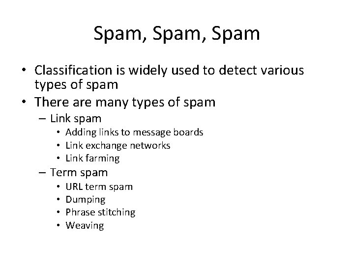
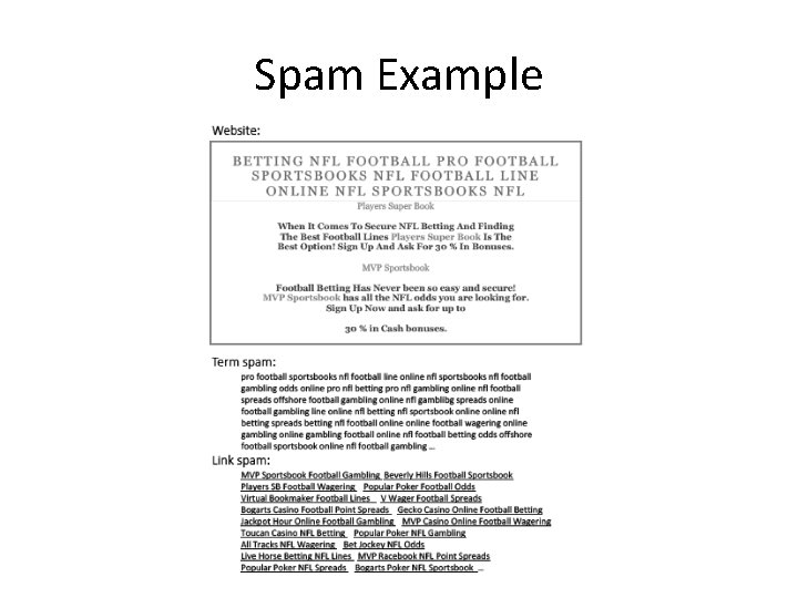
Spam, Spam • Classification is widely used to detect various types of spam • There are many types of spam – Link spam • Adding links to message boards • Link exchange networks • Link farming – Term spam • • URL term spam Dumping Phrase stitching Weaving

Spam Example

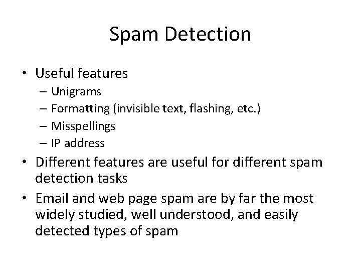
Spam Detection • Useful features – Unigrams – Formatting (invisible text, flashing, etc. ) – Misspellings – IP address • Different features are useful for different spam detection tasks • Email and web page spam are by far the most widely studied, well understood, and easily detected types of spam

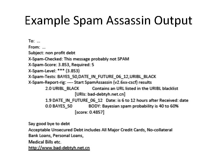
Example Spam Assassin Output

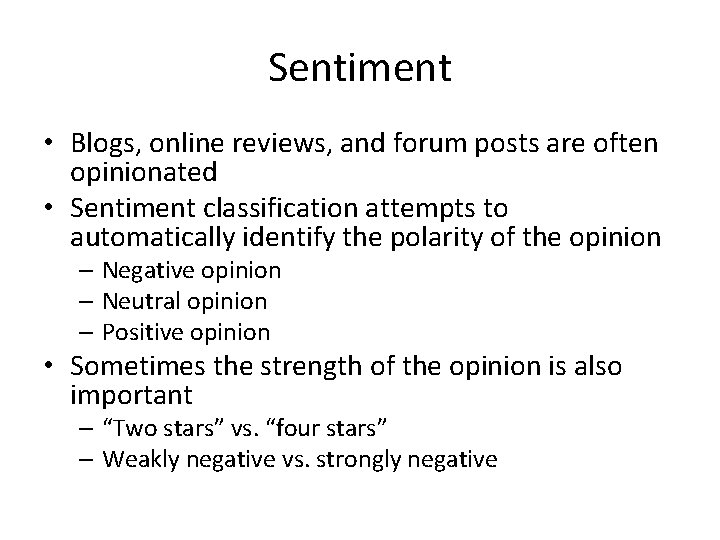
Sentiment • Blogs, online reviews, and forum posts are often opinionated • Sentiment classification attempts to automatically identify the polarity of the opinion – Negative opinion – Neutral opinion – Positive opinion • Sometimes the strength of the opinion is also important – “Two stars” vs. “four stars” – Weakly negative vs. strongly negative

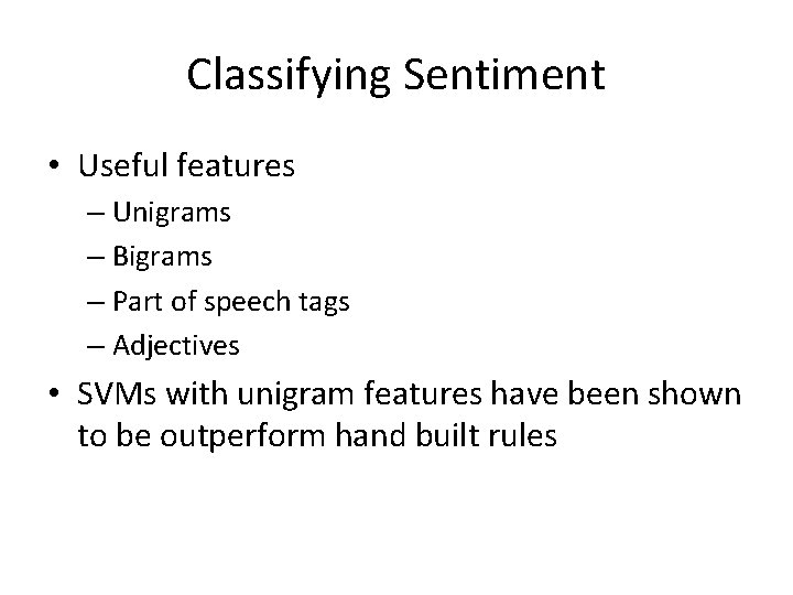
Classifying Sentiment • Useful features – Unigrams – Bigrams – Part of speech tags – Adjectives • SVMs with unigram features have been shown to be outperform hand built rules

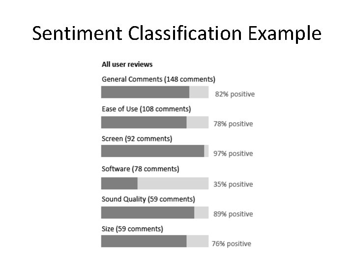
Sentiment Classification Example

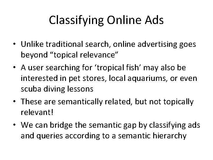
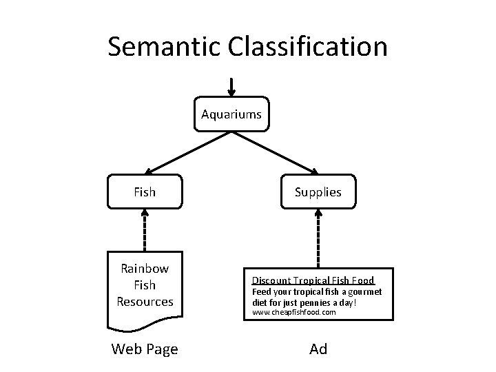
Classifying Online Ads • Unlike traditional search, online advertising goes beyond “topical relevance” • A user searching for ‘tropical fish’ may also be interested in pet stores, local aquariums, or even scuba diving lessons • These are semantically related, but not topically relevant! • We can bridge the semantic gap by classifying ads and queries according to a semantic hierarchy

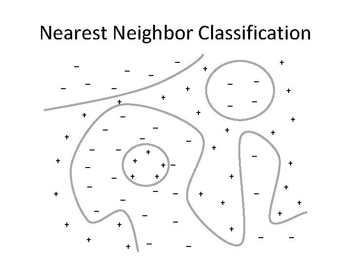
Semantic Classification • Semantic hierarchy ontology – Example: Pets / Aquariums / Supplies • Training data – Large number of queries and ads are manually classified into the hierarchy • Nearest neighbor classification has been shown to be effective for this task • Hierarchical structure of classes can be used to improve classification accuracy

Semantic Classification Aquariums Fish Rainbow Fish Resources Web Page Supplies Discount Tropical Fish Food Feed your tropical fish a gourmet diet for just pennies a day! www. cheapfishfood. com Ad

Clustering • A set of unsupervised algorithms that attempt to find latent structure in a set of items • Goal is to identify groups (clusters) of similar items • Suppose I gave you the shape, color, vitamin C content, and price of various fruits and asked you to cluster them – What criteria would you use? – How would you define similarity? • Clustering is very sensitive to how items are represented and how similarity is defined!

Clustering • General outline of clustering algorithms 1. Decide how items will be represented (e. g. , feature vectors) 2. Define similarity measure between pairs or groups of items (e. g. , cosine similarity) 3. Determine what makes a “good” clustering 4. Iteratively construct clusters that are increasingly “good” 5. Stop after a local/global optimum clustering is found • Steps 3 and 4 differ the most across algorithms

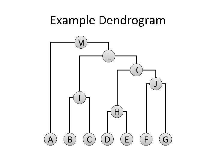
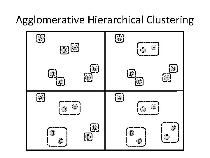
Hierarchical Clustering • Constructs a hierarchy of clusters – The top level of the hierarchy consists of a single cluster with all items in it – The bottom level of the hierarchy consists of N (# items) singleton clusters • Two types of hierarchical clustering – Divisive (“top down”) – Agglomerative (“bottom up”) • Hierarchy can be visualized as a dendogram

Example Dendrogram M L K J I H A B C D E F G

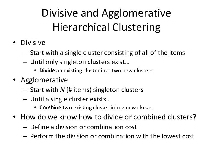
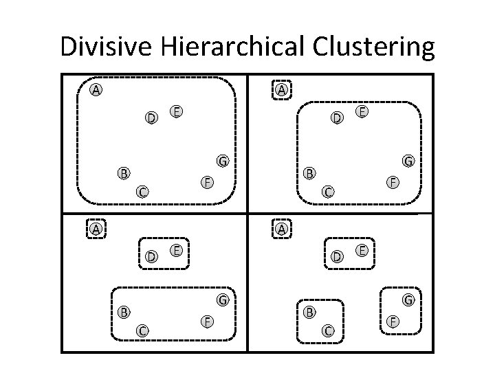
Divisive and Agglomerative Hierarchical Clustering • Divisive – Start with a single cluster consisting of all of the items – Until only singleton clusters exist… • Divide an existing cluster into two new clusters • Agglomerative – Start with N (# items) singleton clusters – Until a single cluster exists… • Combine two existing cluster into a new cluster • How do we know how to divide or combined clusters? – Define a division or combination cost – Perform the division or combination with the lowest cost

Divisive Hierarchical Clustering A A D E D G B F C E F C A A D E D G B C F E G B C F

Agglomerative Hierarchical Clustering A A D E D G B F C E F C A A D E D G B C F E G B C F

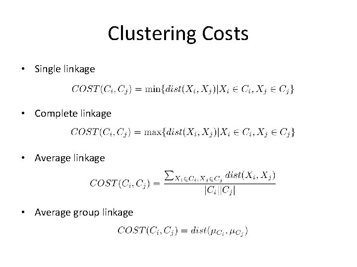
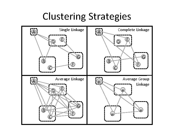
Clustering Costs • Single linkage • Complete linkage • Average group linkage

Clustering Strategies Single Linkage A D E D G B C Average Linkage D E C F F Average Group Linkage μ μ G B E G B F C A Complete Linkage A μ μ

Agglomerative Clustering Algorithm

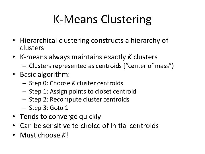
K-Means Clustering • Hierarchical clustering constructs a hierarchy of clusters • K-means always maintains exactly K clusters – Clusters represented as centroids (“center of mass”) • Basic algorithm: – – Step 0: Choose K cluster centroids Step 1: Assign points to closet centroid Step 2: Recompute cluster centroids Step 3: Goto 1 • Tends to converge quickly • Can be sensitive to choice of initial centroids • Must choose K!

K-Means Clustering Algorithm

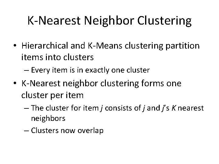
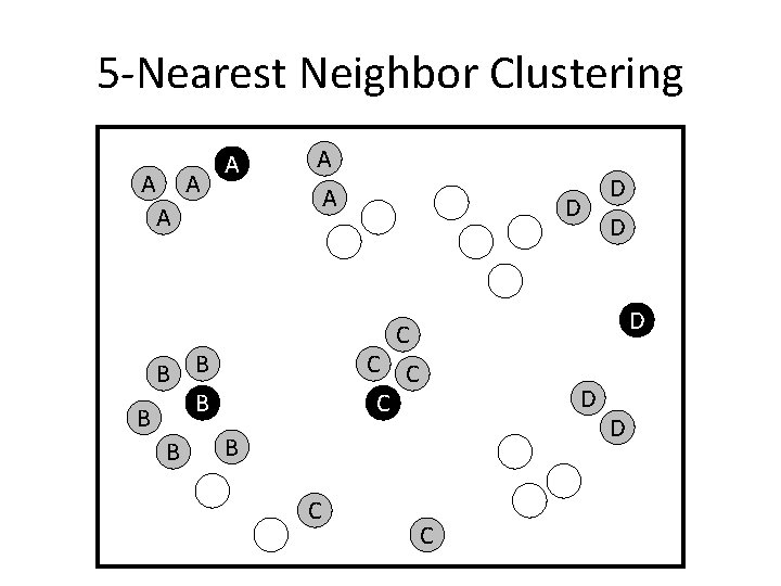
K-Nearest Neighbor Clustering • Hierarchical and K-Means clustering partition items into clusters – Every item is in exactly one cluster • K-Nearest neighbor clustering forms one cluster per item – The cluster for item j consists of j and j’s K nearest neighbors – Clusters now overlap

5 -Nearest Neighbor Clustering A A A B A A A D C C B B D D B C D D C D

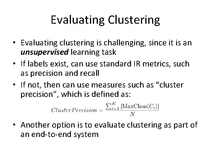
Evaluating Clustering • Evaluating clustering is challenging, since it is an unsupervised learning task • If labels exist, can use standard IR metrics, such as precision and recall • If not, then can use measures such as “cluster precision”, which is defined as: • Another option is to evaluate clustering as part of an end-to-end system

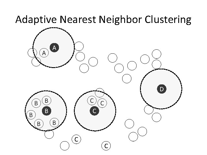
How to Choose K? • K-means and K-nearest neighbor clustering require us to choose K, the number of clusters • No theoretically appealing way of choosing K • Depends on the application and data • Can use hierarchical clustering and choose the best level of the hierarchy to use • Can use adaptive K for K-nearest neighbor clustering – Define a ‘ball’ around each item • Difficult problem with no clear solution

Adaptive Nearest Neighbor Clustering A A D B B B C C C B C C

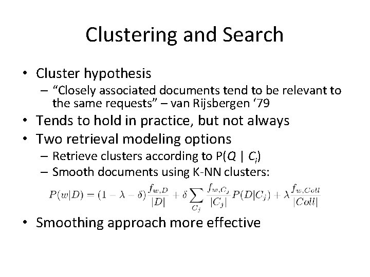
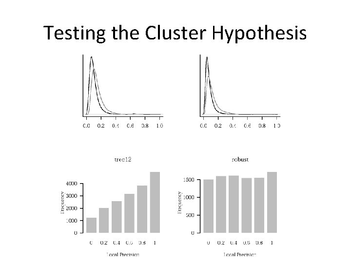
Clustering and Search • Cluster hypothesis – “Closely associated documents tend to be relevant to the same requests” – van Rijsbergen ‘ 79 • Tends to hold in practice, but not always • Two retrieval modeling options – Retrieve clusters according to P(Q | Ci) – Smooth documents using K-NN clusters: • Smoothing approach more effective

Testing the Cluster Hypothesis