Search Engines Information Retrieval in Practice All slides

Search Engines Information Retrieval in Practice All slides ©Addison Wesley, 2008 1

Retrieval Models • Provide a mathematical framework for defining the search process – includes explanation of assumptions – basis of many ranking algorithms – can be implicit • Progress in retrieval models has corresponded with improvements in effectiveness • Theories about relevance 2

Relevance • Complex concept that has been studied for some time – Many factors to consider – People often disagree when making relevance judgments • Retrieval models make various assumptions about relevance to simplify problem – e. g. , topical vs. user relevance – e. g. , binary vs. multi-valued relevance 3

Retrieval Model Overview • Older models – Boolean retrieval – Vector Space model • Probabilistic Models – BM 25 – Language models • Combining evidence – Inference networks – Learning to Rank 4

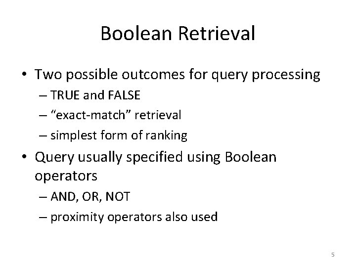
Boolean Retrieval • Two possible outcomes for query processing – TRUE and FALSE – “exact-match” retrieval – simplest form of ranking • Query usually specified using Boolean operators – AND, OR, NOT – proximity operators also used 5

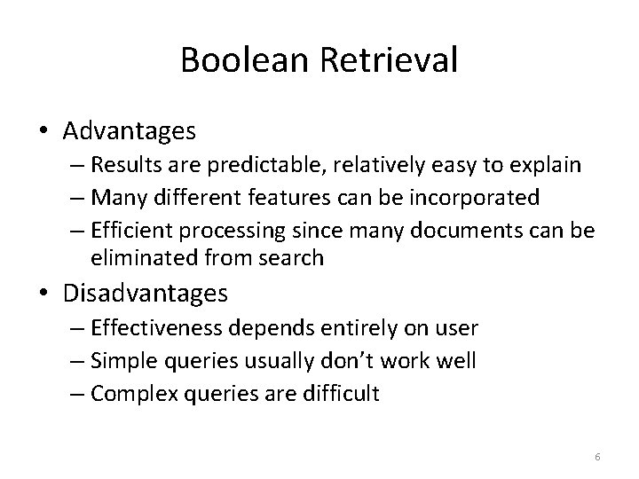
Boolean Retrieval • Advantages – Results are predictable, relatively easy to explain – Many different features can be incorporated – Efficient processing since many documents can be eliminated from search • Disadvantages – Effectiveness depends entirely on user – Simple queries usually don’t work well – Complex queries are difficult 6

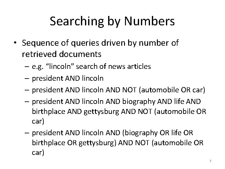
Searching by Numbers • Sequence of queries driven by number of retrieved documents – e. g. “lincoln” search of news articles – president AND lincoln AND NOT (automobile OR car) – president AND lincoln AND biography AND life AND birthplace AND gettysburg AND NOT (automobile OR car) – president AND lincoln AND (biography OR life OR birthplace OR gettysburg) AND NOT (automobile OR car) 7

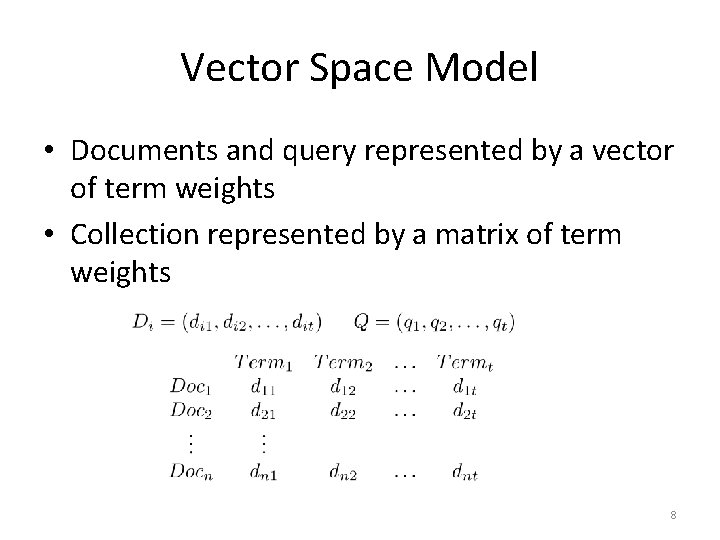
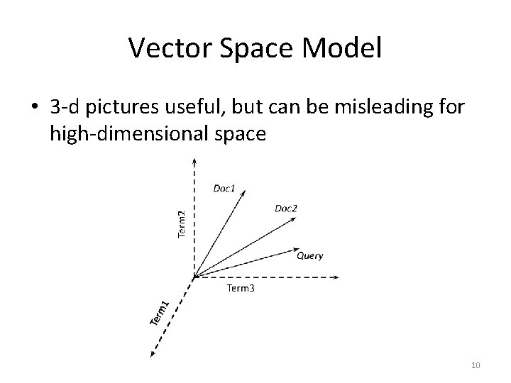
Vector Space Model • Documents and query represented by a vector of term weights • Collection represented by a matrix of term weights 8

Vector Space Model 9

Vector Space Model • 3 -d pictures useful, but can be misleading for high-dimensional space 10

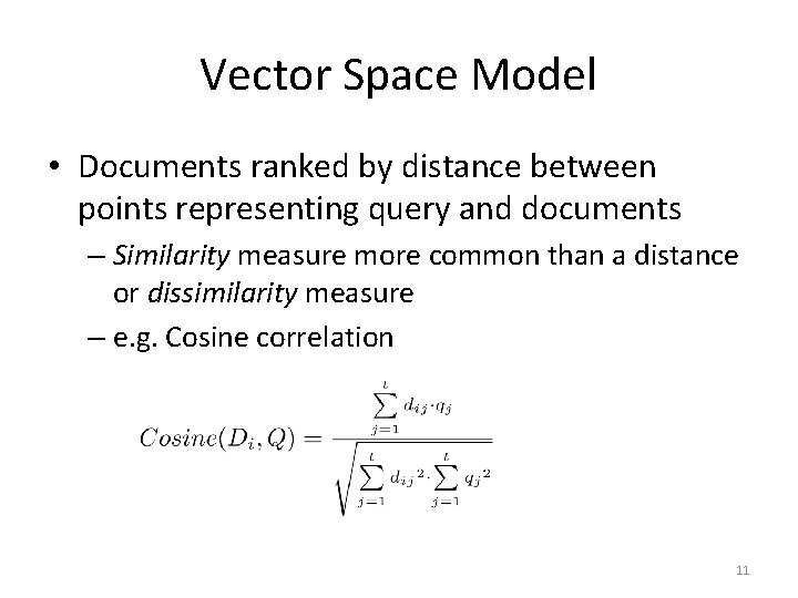
Vector Space Model • Documents ranked by distance between points representing query and documents – Similarity measure more common than a distance or dissimilarity measure – e. g. Cosine correlation 11

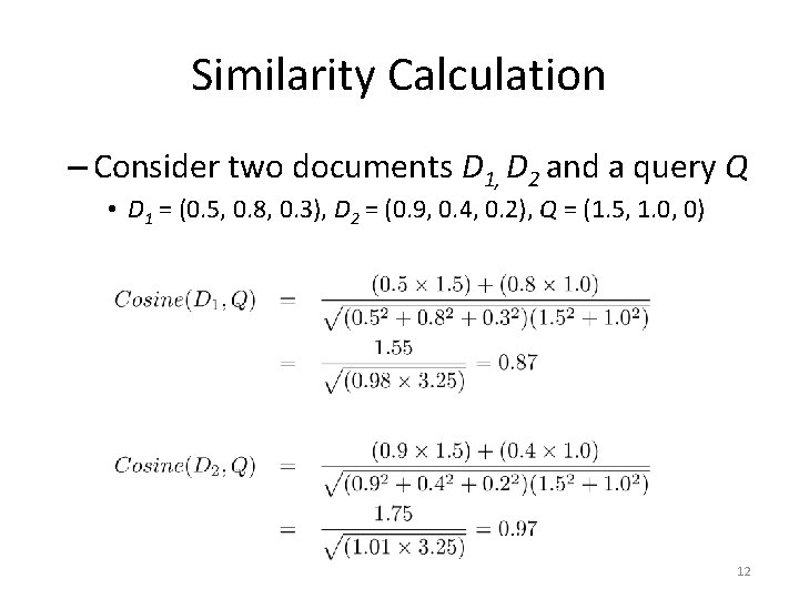
Similarity Calculation – Consider two documents D 1, D 2 and a query Q • D 1 = (0. 5, 0. 8, 0. 3), D 2 = (0. 9, 0. 4, 0. 2), Q = (1. 5, 1. 0, 0) 12

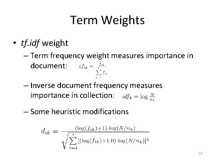
Term Weights • tf. idf weight – Term frequency weight measures importance in document: – Inverse document frequency measures importance in collection: – Some heuristic modifications 13

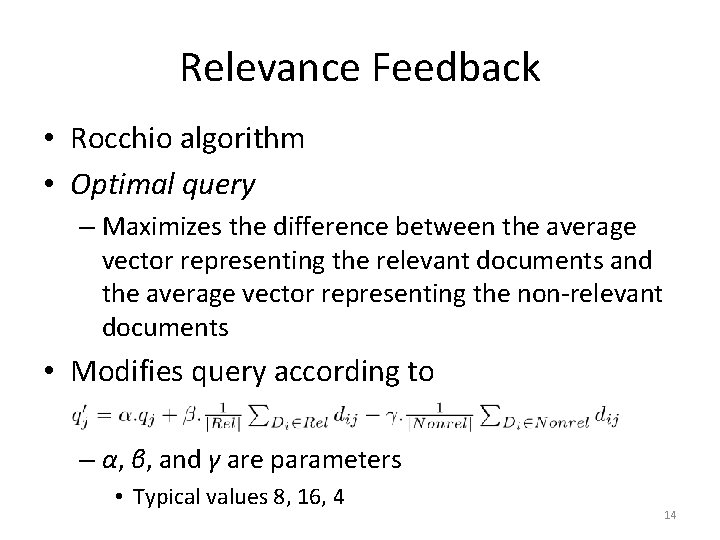
Relevance Feedback • Rocchio algorithm • Optimal query – Maximizes the difference between the average vector representing the relevant documents and the average vector representing the non-relevant documents • Modifies query according to – α, β, and γ are parameters • Typical values 8, 16, 4 14

Vector Space Model • Advantages – Simple computational framework for ranking – Any similarity measure or term weighting scheme could be used • Disadvantages – Assumption of term independence – No predictions about techniques for effective ranking 15

Probability Ranking Principle • Robertson (1977) – “If a reference retrieval system’s response to each request is a ranking of the documents in the collection in order of decreasing probability of relevance to the user who submitted the request, – where the probabilities are estimated as accurately as possible on the basis of whatever data have been made available to the system for this purpose, – the overall effectiveness of the system to its user will be the best that is obtainable on the basis of those data. ” 16

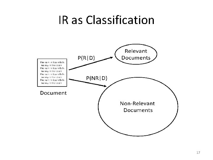
IR as Classification 17

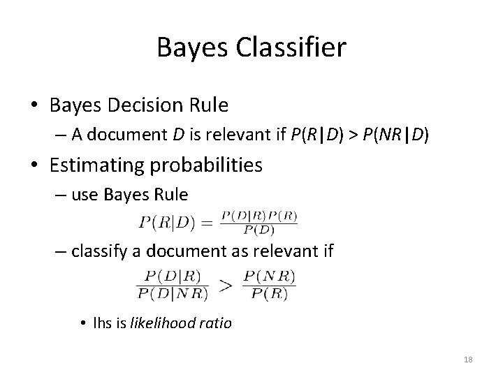
Bayes Classifier • Bayes Decision Rule – A document D is relevant if P(R|D) > P(NR|D) • Estimating probabilities – use Bayes Rule – classify a document as relevant if • lhs is likelihood ratio 18

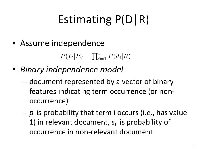
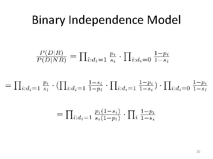
Estimating P(D|R) • Assume independence • Binary independence model – document represented by a vector of binary features indicating term occurrence (or nonoccurrence) – pi is probability that term i occurs (i. e. , has value 1) in relevant document, si is probability of occurrence in non-relevant document 19

Binary Independence Model 20

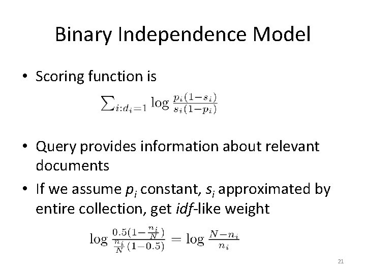
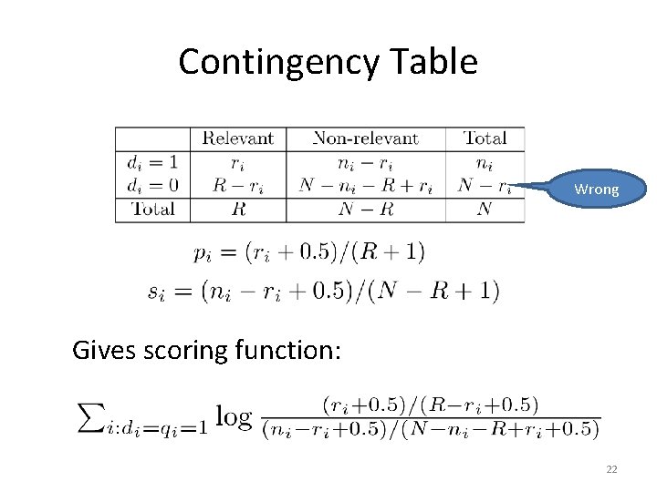
Binary Independence Model • Scoring function is • Query provides information about relevant documents • If we assume pi constant, si approximated by entire collection, get idf-like weight 21

Contingency Table Wrong Gives scoring function: 22

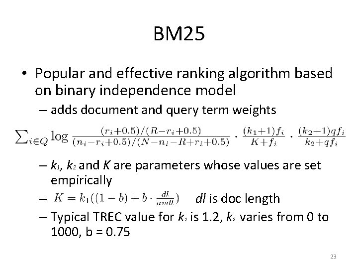
BM 25 • Popular and effective ranking algorithm based on binary independence model – adds document and query term weights – k 1, k 2 and K are parameters whose values are set empirically – dl is doc length – Typical TREC value for k is 1. 2, k varies from 0 to 1000, b = 0. 75 1 2 23

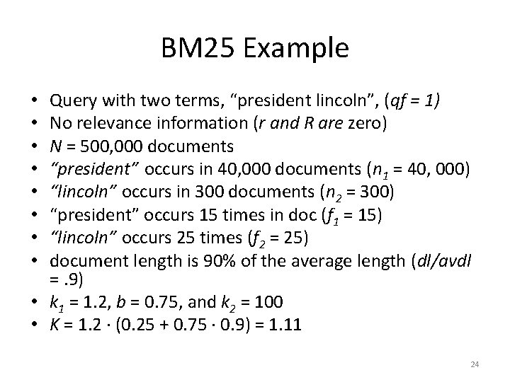
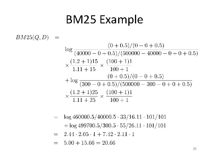
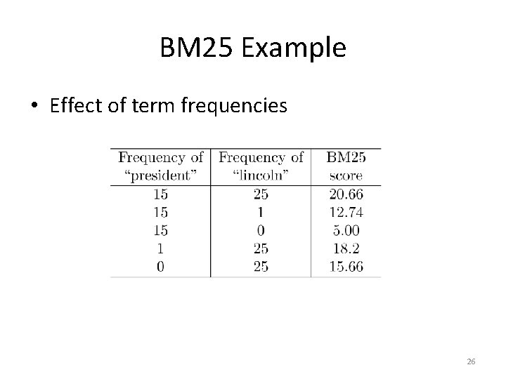
BM 25 Example Query with two terms, “president lincoln”, (qf = 1) No relevance information (r and R are zero) N = 500, 000 documents “president” occurs in 40, 000 documents (n 1 = 40, 000) “lincoln” occurs in 300 documents (n 2 = 300) “president” occurs 15 times in doc (f 1 = 15) “lincoln” occurs 25 times (f 2 = 25) document length is 90% of the average length (dl/avdl =. 9) • k 1 = 1. 2, b = 0. 75, and k 2 = 100 • K = 1. 2 · (0. 25 + 0. 75 · 0. 9) = 1. 11 • • 24

BM 25 Example 25

BM 25 Example • Effect of term frequencies 26

Language Model • Unigram language model – probability distribution over the words in a language – generation of text consists of pulling words out of a “bucket” according to the probability distribution and replacing them • N-gram language model – some applications use bigram and trigram language models where probabilities depend on previous words 27

Language Model • A topic in a document or query can be represented as a language model – i. e. , words that tend to occur often when discussing a topic will have high probabilities in the corresponding language model • Multinomial distribution over words – text is modeled as a finite sequence of words, where there are t possible words at each point in the sequence – commonly used, but not only possibility – doesn’t model burstiness 28

LMs for Retrieval • 3 possibilities: – probability of generating the query text from a document language model – probability of generating the document text from a query language model – comparing the language models representing the query and document topics • Models of topical relevance 29

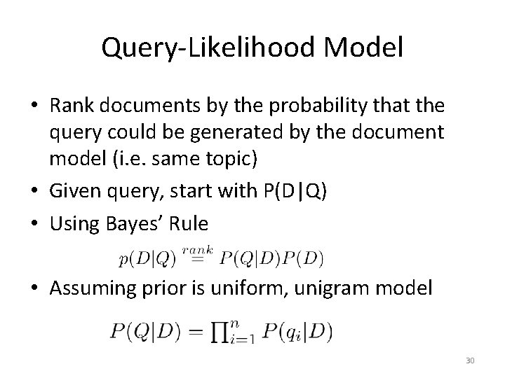
Query-Likelihood Model • Rank documents by the probability that the query could be generated by the document model (i. e. same topic) • Given query, start with P(D|Q) • Using Bayes’ Rule • Assuming prior is uniform, unigram model 30

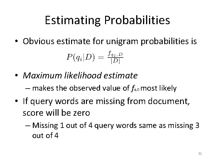
Estimating Probabilities • Obvious estimate for unigram probabilities is • Maximum likelihood estimate – makes the observed value of fq ; D most likely i • If query words are missing from document, score will be zero – Missing 1 out of 4 query words same as missing 3 out of 4 31

Smoothing • Document texts are a sample from the language model – Missing words should not have zero probability of occurring • Smoothing is a technique for estimating probabilities for missing (or unseen) words – lower (or discount) the probability estimates for words that are seen in the document text – assign that “left-over” probability to the estimates for the words that are not seen in the text 32

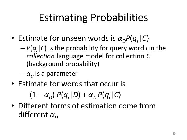
Estimating Probabilities • Estimate for unseen words is αDP(qi|C) – P(qi|C) is the probability for query word i in the collection language model for collection C (background probability) – αD is a parameter • Estimate for words that occur is (1 − αD) P(qi|D) + αD P(qi|C) • Different forms of estimation come from different αD 33

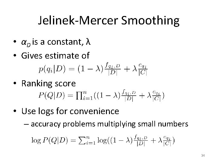
Jelinek-Mercer Smoothing • αD is a constant, λ • Gives estimate of • Ranking score • Use logs for convenience – accuracy problems multiplying small numbers 34

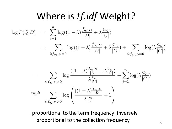
Where is tf. idf Weight? - proportional to the term frequency, inversely proportional to the collection frequency 35

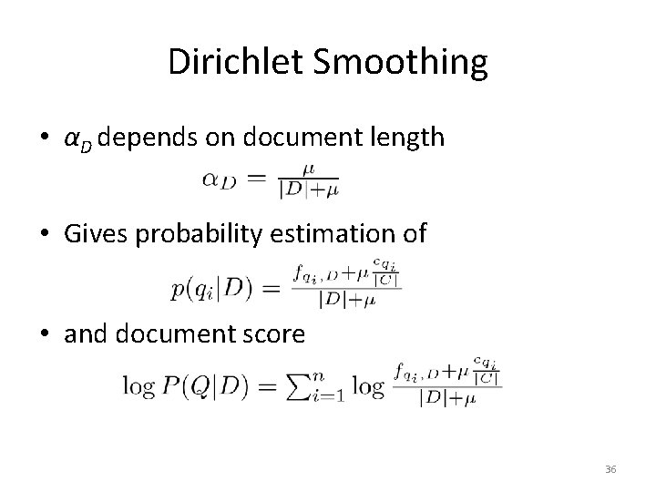
Dirichlet Smoothing • αD depends on document length • Gives probability estimation of • and document score 36

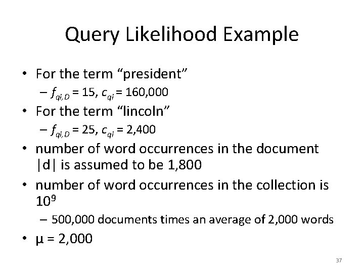
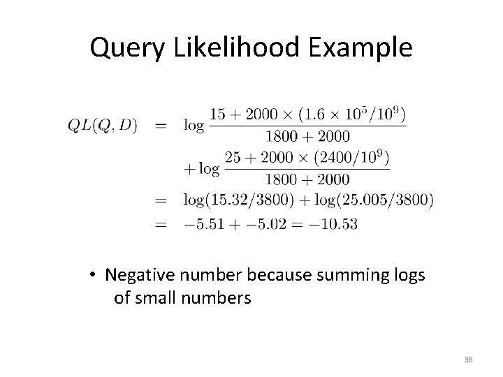
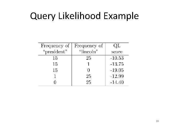
Query Likelihood Example • For the term “president” – fqi, D = 15, cqi = 160, 000 • For the term “lincoln” – fqi, D = 25, cqi = 2, 400 • number of word occurrences in the document |d| is assumed to be 1, 800 • number of word occurrences in the collection is 109 – 500, 000 documents times an average of 2, 000 words • μ = 2, 000 37

Query Likelihood Example • Negative number because summing logs of small numbers 38

Query Likelihood Example 39

Relevance Models • Relevance model – language model representing information need – query and relevant documents are samples from this model • P(D|R) - probability of generating the text in a document given a relevance model – document likelihood model – less effective than query likelihood due to difficulties comparing across documents of different lengths 40

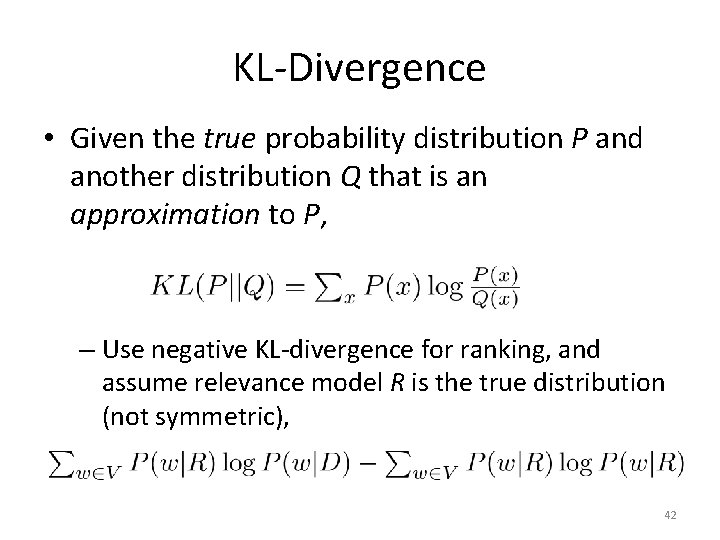
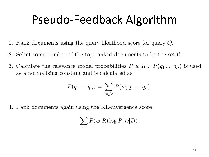
Pseudo-Relevance Feedback • Estimate relevance model from query and topranked documents • Rank documents by similarity of document model to relevance model • Kullback-Leibler divergence (KL-divergence) is a well-known measure of the difference between two probability distributions 41

KL-Divergence • Given the true probability distribution P and another distribution Q that is an approximation to P, – Use negative KL-divergence for ranking, and assume relevance model R is the true distribution (not symmetric), 42

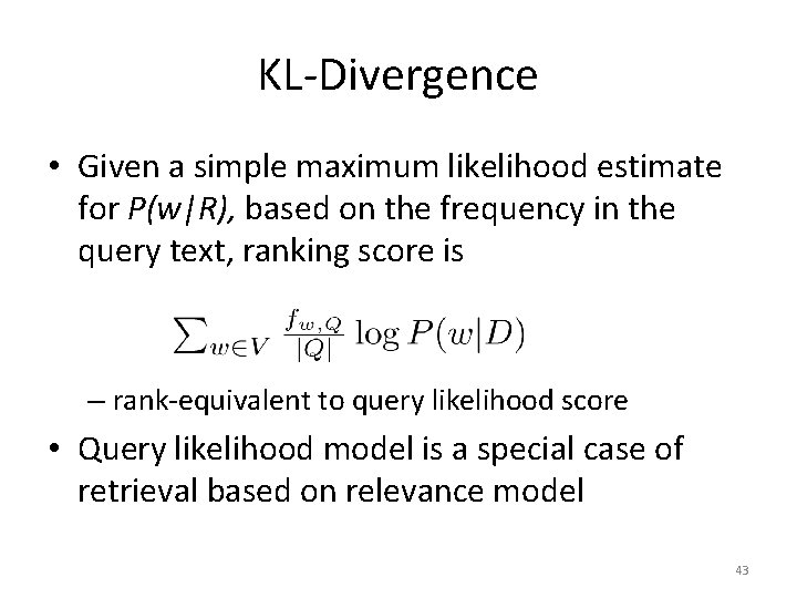
KL-Divergence • Given a simple maximum likelihood estimate for P(w|R), based on the frequency in the query text, ranking score is – rank-equivalent to query likelihood score • Query likelihood model is a special case of retrieval based on relevance model 43

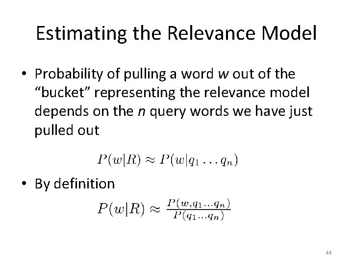
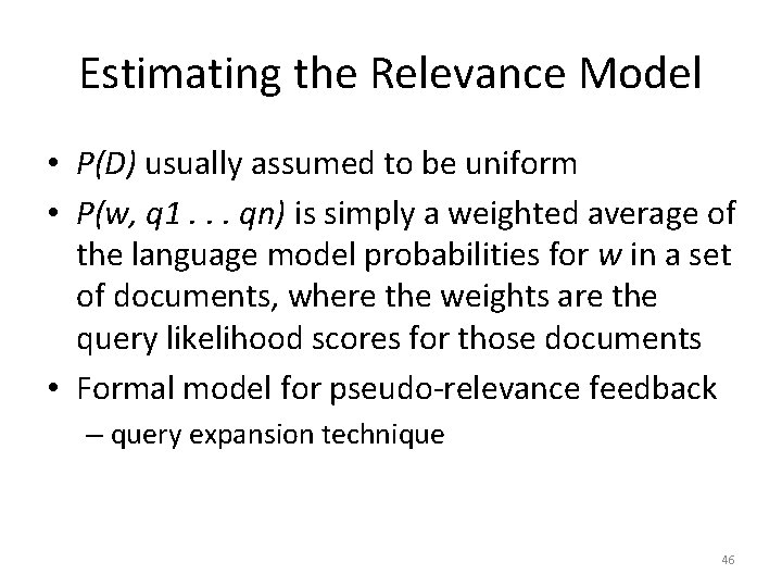
Estimating the Relevance Model • Probability of pulling a word w out of the “bucket” representing the relevance model depends on the n query words we have just pulled out • By definition 44

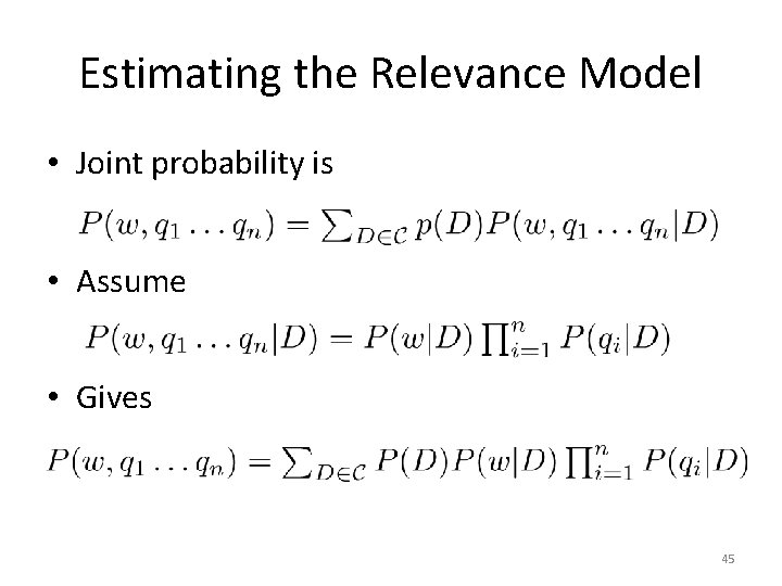
Estimating the Relevance Model • Joint probability is • Assume • Gives 45

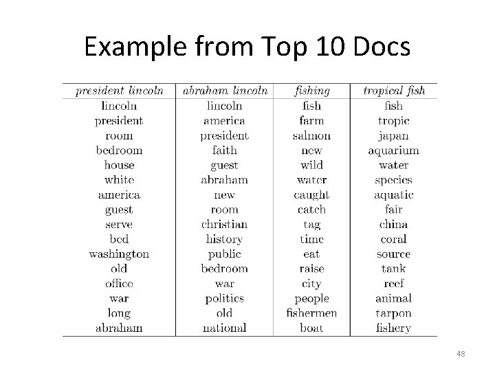
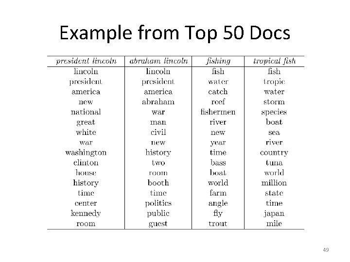
Estimating the Relevance Model • P(D) usually assumed to be uniform • P(w, q 1. . . qn) is simply a weighted average of the language model probabilities for w in a set of documents, where the weights are the query likelihood scores for those documents • Formal model for pseudo-relevance feedback – query expansion technique 46

Pseudo-Feedback Algorithm 47

Example from Top 10 Docs 48

Example from Top 50 Docs 49

Combining Evidence • Effective retrieval requires the combination of many pieces of evidence about a document’s potential relevance – have focused on simple word-based evidence – many other types of evidence • structure, Page. Rank, metadata, even scores from different models • Inference network model is one approach to combining evidence – uses Bayesian network formalism 50

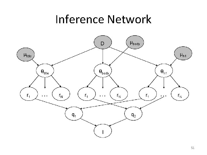
Inference Network 51

Inference Network • Document node (D) corresponds to the event that a document is observed • Representation nodes (ri) are document features (evidence) – Probabilities associated with those features are based on language models θ estimated using the parameters μ – one language model for each significant document structure – ri nodes can represent proximity features, or other types of evidence (e. g. date) 52

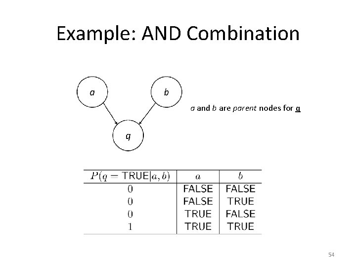
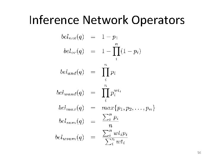
Inference Network • Query nodes (qi) are used to combine evidence from representation nodes and other query nodes – represent the occurrence of more complex evidence and document features – a number of combination operators are available • Information need node (I) is a special query node that combines all of the evidence from the other query nodes – network computes P(I|D, μ) 53

Example: AND Combination a and b are parent nodes for q 54

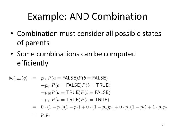
Example: AND Combination • Combination must consider all possible states of parents • Some combinations can be computed efficiently 55

Inference Network Operators 56

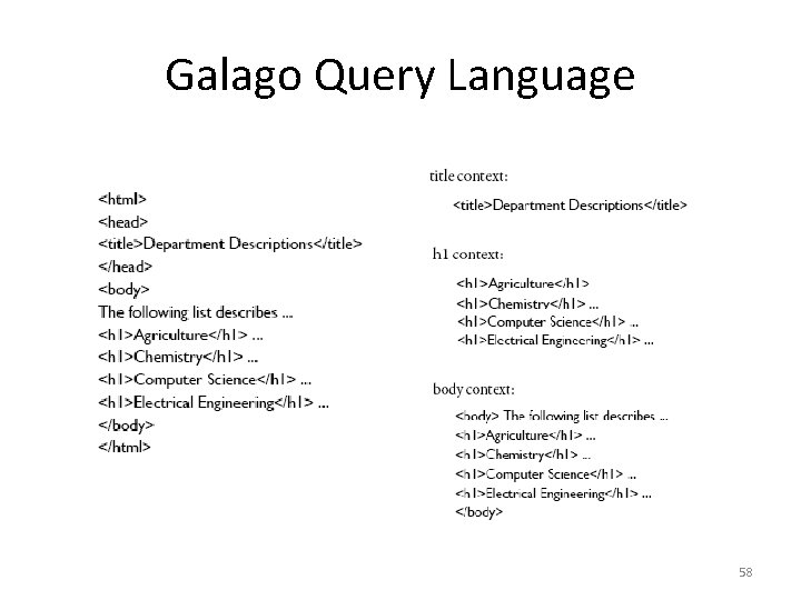
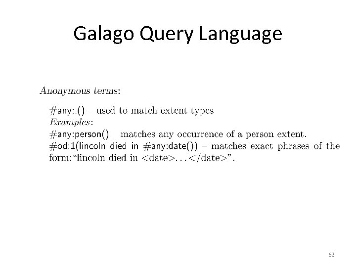
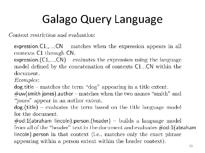
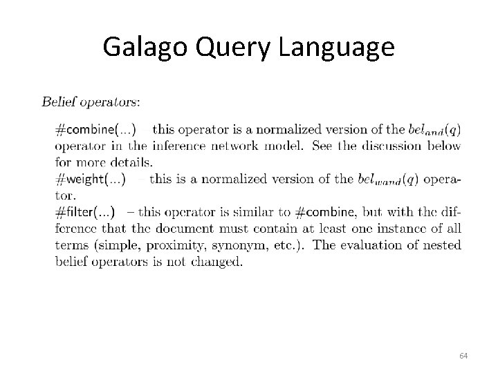
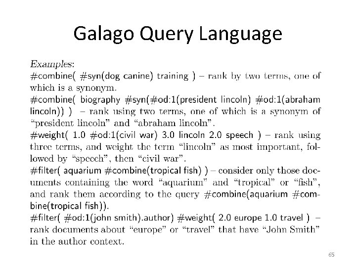
Galago Query Language • A document is viewed as a sequence of text that may contain arbitrary tags • A single context is generated for each unique tag name • An extent is a sequence of text that appears within a single begin/end tag pair of the same type as the context 57

Galago Query Language 58

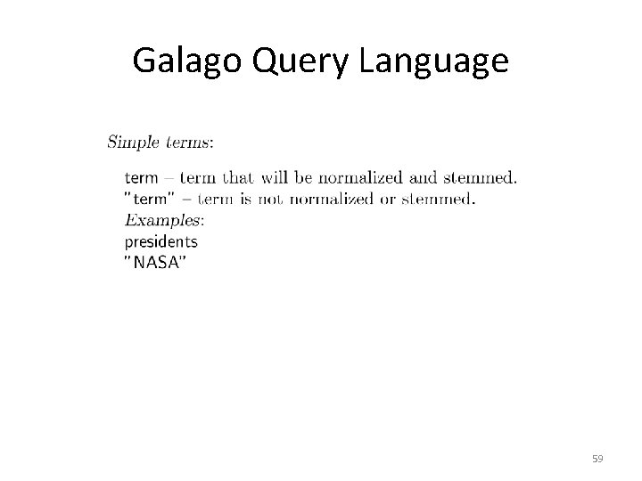
Galago Query Language Tex. Point Display 59

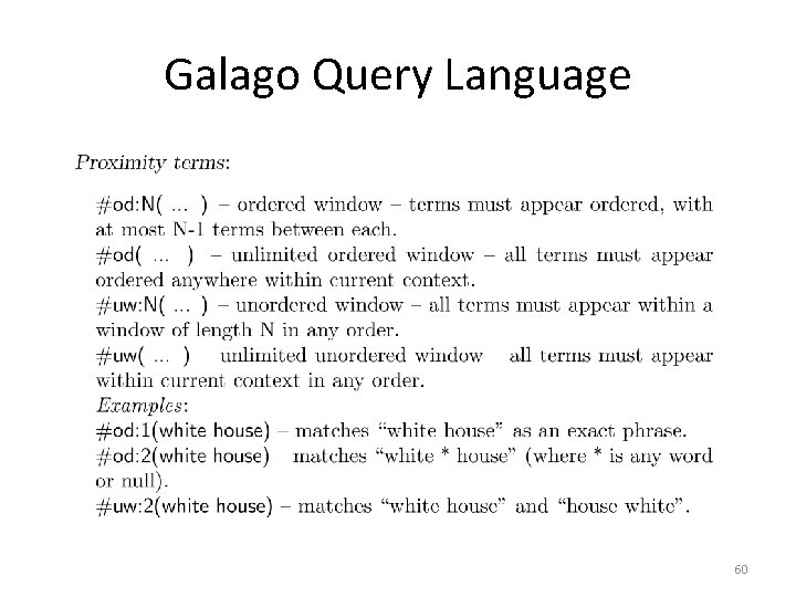
Galago Query Language 60

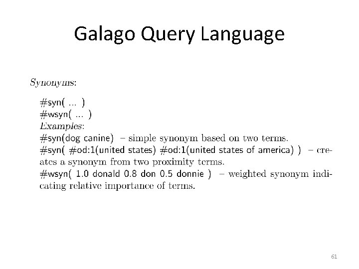
Galago Query Language 61

Galago Query Language 62

Galago Query Language 63

Galago Query Language 64

Galago Query Language 65

Web Search • Most important, but not only, search application • Major differences to TREC news – Size of collection – Connections between documents – Range of document types – Importance of spam – Volume of queries – Range of query types 66

Search Taxonomy • Informational – Finding information about some topic which may be on one or more web pages – Topical search • Navigational – finding a particular web page that the user has either seen before or is assumed to exist • Transactional – finding a site where a task such as shopping or downloading music can be performed 67

Web Search • For effective navigational and transactional search, need to combine features that reflect user relevance • Commercial web search engines combine evidence from hundreds of features to generate a ranking score for a web page – page content, page metadata, anchor text, links (e. g. , Page. Rank), and user behavior (click logs) – page metadata – e. g. , “age”, how often it is updated, the URL of the page, the domain name of its site, and the amount of text content 68

Search Engine Optimization • SEO: understanding the relative importance of features used in search and how they can be manipulated to obtain better search rankings for a web page – e. g. , improve the text used in the title tag, improve the text in heading tags, make sure that the domain name and URL contain important keywords, and try to improve the anchor text and link structure – Some of these techniques are regarded as not appropriate by search engine companies 69

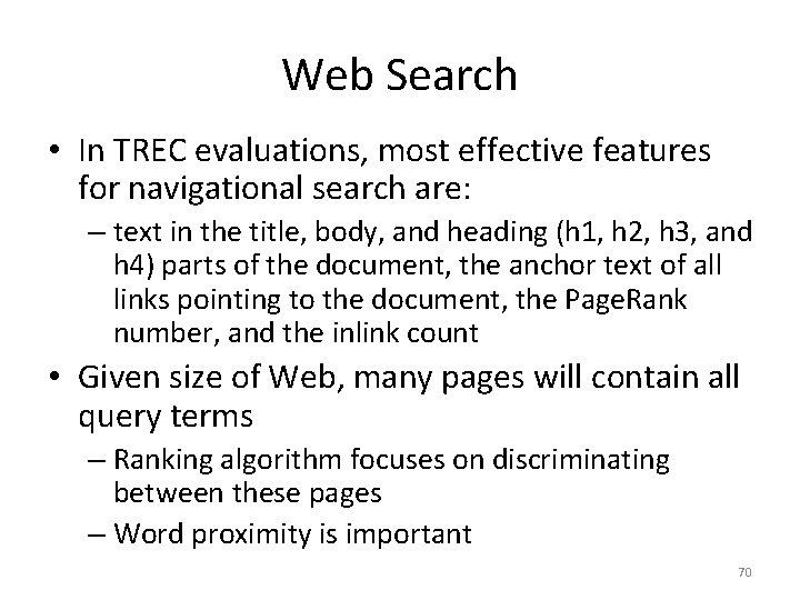
Web Search • In TREC evaluations, most effective features for navigational search are: – text in the title, body, and heading (h 1, h 2, h 3, and h 4) parts of the document, the anchor text of all links pointing to the document, the Page. Rank number, and the inlink count • Given size of Web, many pages will contain all query terms – Ranking algorithm focuses on discriminating between these pages – Word proximity is important 70

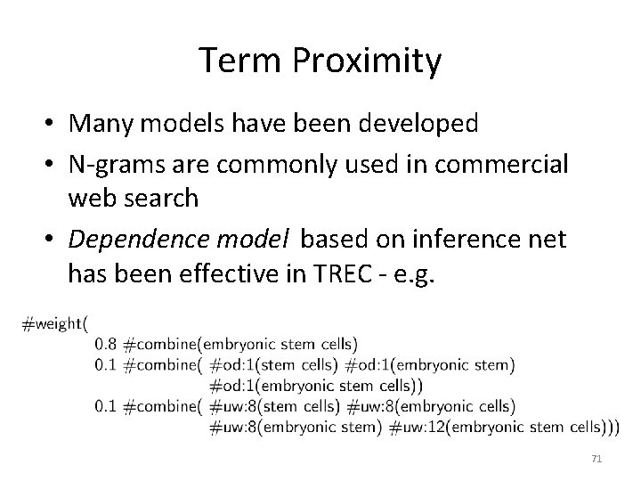
Term Proximity • Many models have been developed • N-grams are commonly used in commercial web search • Dependence model based on inference net has been effective in TREC - e. g. 71

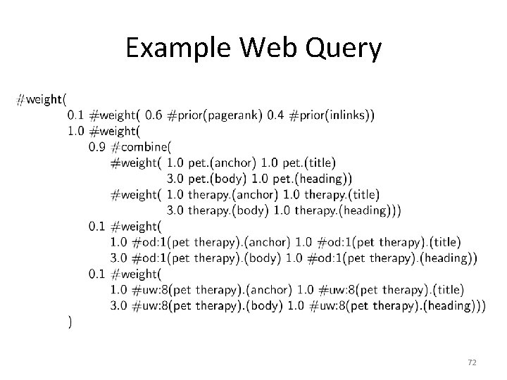
Example Web Query 72

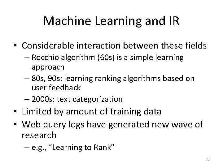
Machine Learning and IR • Considerable interaction between these fields – Rocchio algorithm (60 s) is a simple learning approach – 80 s, 90 s: learning ranking algorithms based on user feedback – 2000 s: text categorization • Limited by amount of training data • Web query logs have generated new wave of research – e. g. , “Learning to Rank” 73

Generative vs. Discriminative • All of the probabilistic retrieval models presented so far fall into the category of generative models – A generative model assumes that documents were generated from some underlying model (in this case, usually a multinomial distribution) and uses training data to estimate the parameters of the model – probability of belonging to a class (i. e. the relevant documents for a query) is then estimated using Bayes’ Rule and the document model 74

Generative vs. Discriminative • A discriminative model estimates the probability of belonging to a class directly from the observed features of the document based on the training data • Generative models perform well with low numbers of training examples • Discriminative models usually have the advantage given enough training data – Can also easily incorporate many features 75

Discriminative Models for IR • Discriminative models can be trained using explicit relevance judgments or click data in query logs – Click data is much cheaper, more noisy – e. g. Ranking Support Vector Machine (SVM) takes as input partial rank information for queries • partial information about which documents should be ranked higher than others 76

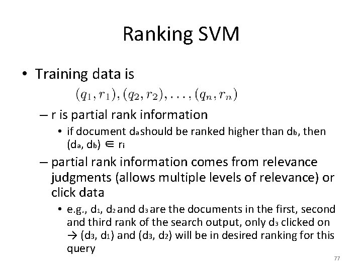
Ranking SVM • Training data is – r is partial rank information • if document da should be ranked higher than db, then (da, db) ∈ ri – partial rank information comes from relevance judgments (allows multiple levels of relevance) or click data • e. g. , d 1, d 2 and d 3 are the documents in the first, second and third rank of the search output, only d 3 clicked on → (d 3, d 1) and (d 3, d 2) will be in desired ranking for this query 77

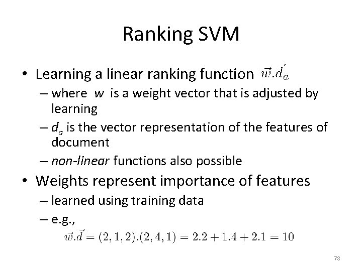
Ranking SVM • Learning a linear ranking function – where w is a weight vector that is adjusted by learning – da is the vector representation of the features of document – non-linear functions also possible • Weights represent importance of features – learned using training data – e. g. , 78

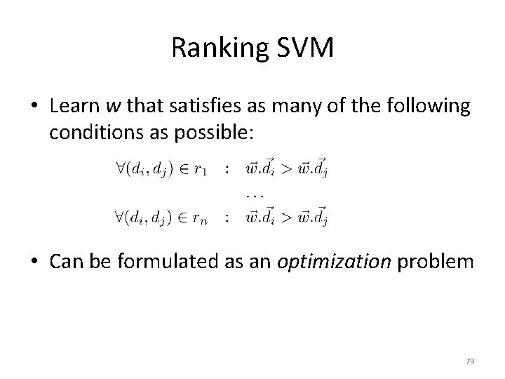
Ranking SVM • Learn w that satisfies as many of the following conditions as possible: • Can be formulated as an optimization problem 79

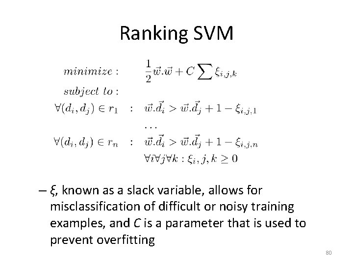
Ranking SVM – ξ, known as a slack variable, allows for misclassification of difficult or noisy training examples, and C is a parameter that is used to prevent overfitting 80

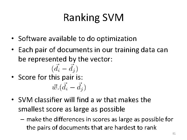
Ranking SVM • Software available to do optimization • Each pair of documents in our training data can be represented by the vector: • Score for this pair is: • SVM classifier will find a w that makes the smallest score as large as possible – make the differences in scores as large as possible for the pairs of documents that are hardest to rank 81

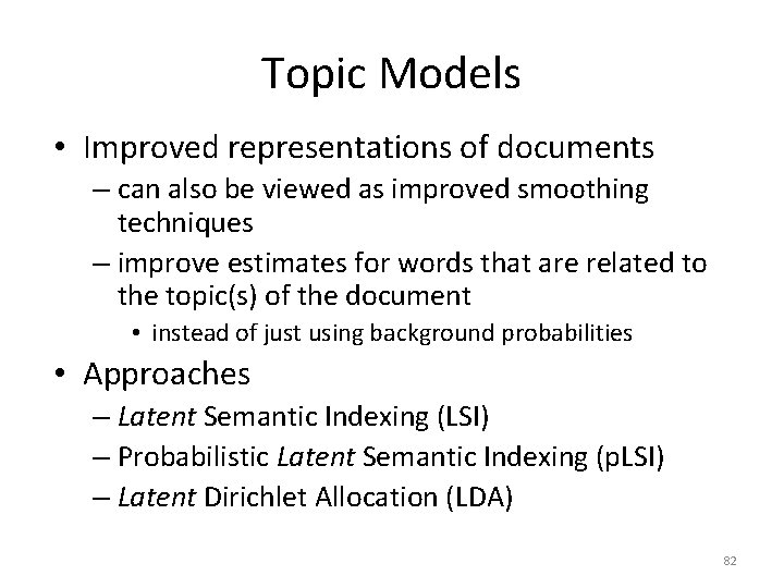
Topic Models • Improved representations of documents – can also be viewed as improved smoothing techniques – improve estimates for words that are related to the topic(s) of the document • instead of just using background probabilities • Approaches – Latent Semantic Indexing (LSI) – Probabilistic Latent Semantic Indexing (p. LSI) – Latent Dirichlet Allocation (LDA) 82

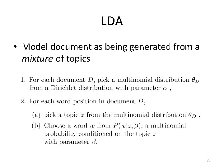
LDA • Model document as being generated from a mixture of topics 83

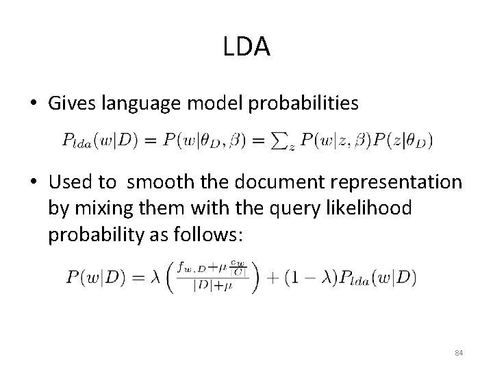
LDA • Gives language model probabilities • Used to smooth the document representation by mixing them with the query likelihood probability as follows: 84

LDA • If the LDA probabilities are used directly as the document representation, the effectiveness will be significantly reduced because the features are too smoothed – e. g. , in typical TREC experiment, only 400 topics used for the entire collection – generating LDA topics is expensive • When used for smoothing, effectiveness is improved 85

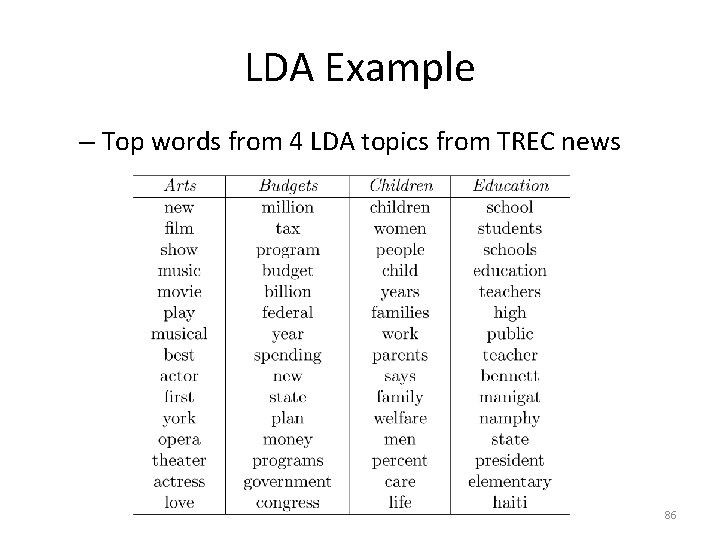
LDA Example – Top words from 4 LDA topics from TREC news 86

Summary • Best retrieval model depends on application and data available • Evaluation corpus (or test collection), training data, and user data are all critical resources • Open source search engines can be used to find effective ranking algorithms – Galago query language makes this particularly easy • Language resources (e. g. , thesaurus) can make a big difference 87