
Search cont CSP Intro Tamara Berg CS 560

Search (cont) & CSP Intro Tamara Berg CS 560 Artificial Intelligence Many slides throughout the course adapted from Dan Klein, Stuart Russell, Andrew Moore, Svetlana Lazebnik, Percy Liang, Luke Zettlemoyer

Reminders • HW 1 is due Sept 10 – This will take a significant amount of time. Start now! – Anyone still looking for a group?
Recall from last class

Uninformed search
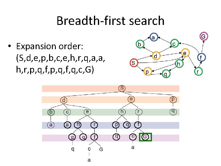
Breadth-first search • Expansion order: (S, d, e, p, b, c, e, h, r, q, a, a, h, r, p, q, f, q, c, G)
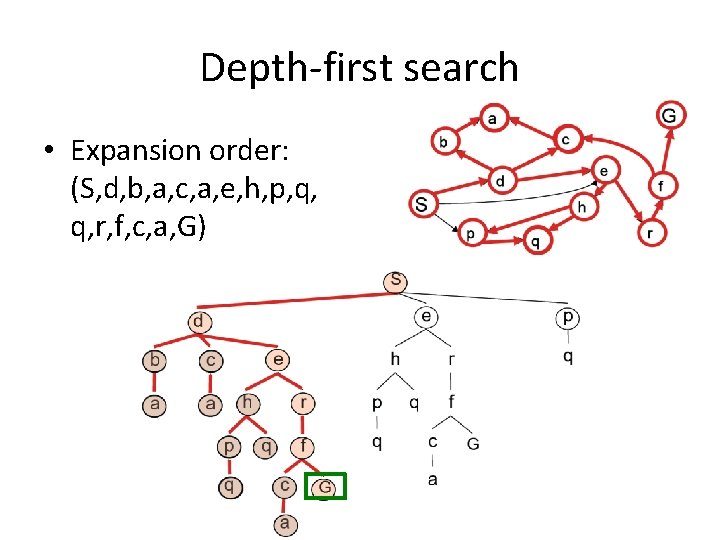
Depth-first search • Expansion order: (S, d, b, a, c, a, e, h, p, q, q, r, f, c, a, G)
Properties of breadth-first search • Complete? Yes (if branching factor b is finite) • Optimal? Not generally – the shallowest goal node is not necessarily the optimal one Yes – if all actions have same cost • Time? Number of nodes in a b-ary tree of depth d: O(bd) (d is the depth of the optimal solution) • Space? O(bd)
Properties of depth-first search • Complete? Fails in infinite-depth spaces, spaces with loops Modify to avoid repeated states along path complete in finite spaces • Optimal? No – returns the first solution it finds • Time? May generate all of the O(bm) nodes, m=max depth of any node Terrible if m is much larger than d • Space? O(bm), i. e. , linear space!
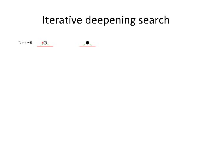
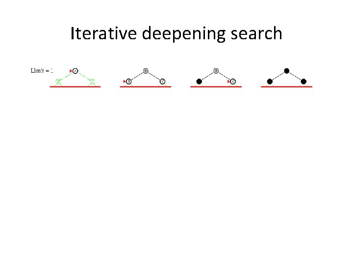
Iterative deepening search • Use DFS as a subroutine 1. Check the root 2. Do a DFS with depth limit 1 3. If there is no path of length 1, do a DFS search with depth limit 2 4. If there is no path of length 2, do a DFS with depth limit 3. 5. And so on…
Iterative deepening search
Iterative deepening search
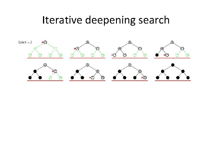
Iterative deepening search
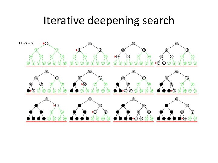
Iterative deepening search
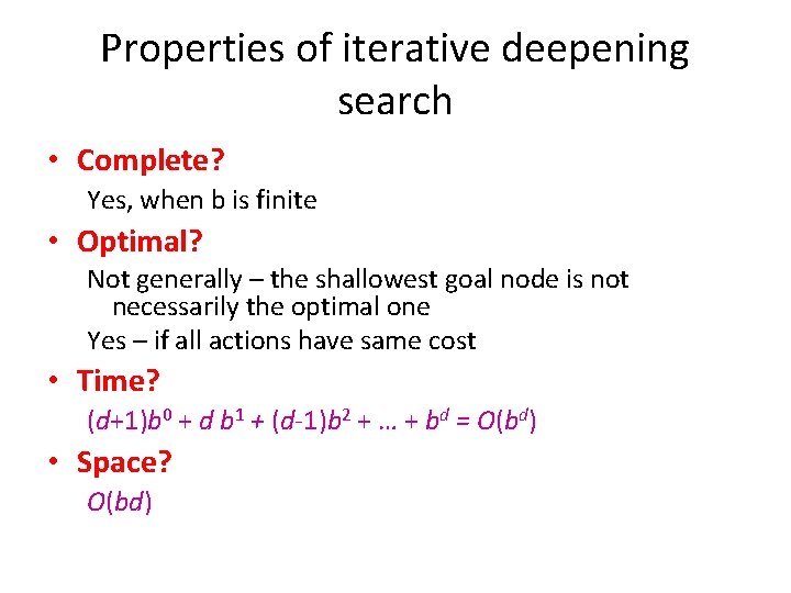
Properties of iterative deepening search • Complete? Yes, when b is finite • Optimal? Not generally – the shallowest goal node is not necessarily the optimal one Yes – if all actions have same cost • Time? (d+1)b 0 + d b 1 + (d-1)b 2 + … + bd = O(bd) • Space? O(bd)
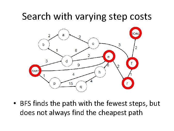
Search with varying step costs • BFS finds the path with the fewest steps, but does not always find the cheapest path
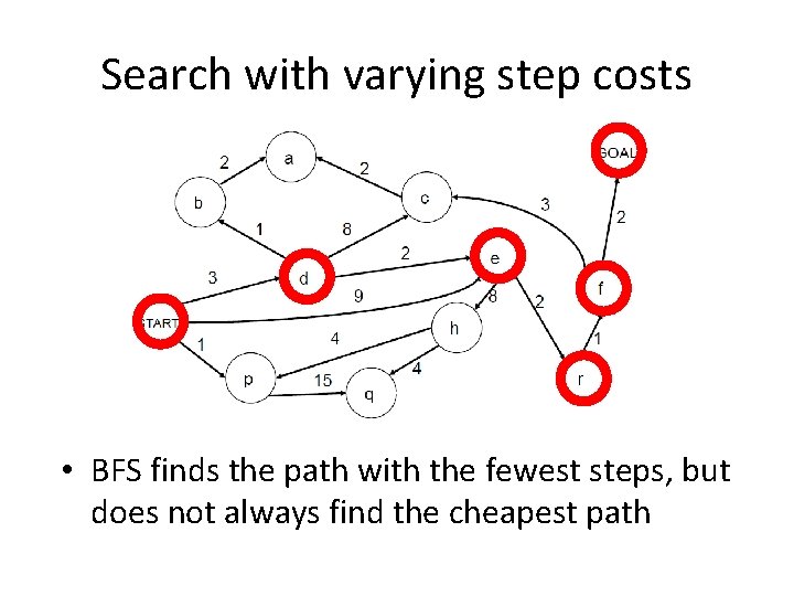
Search with varying step costs • BFS finds the path with the fewest steps, but does not always find the cheapest path
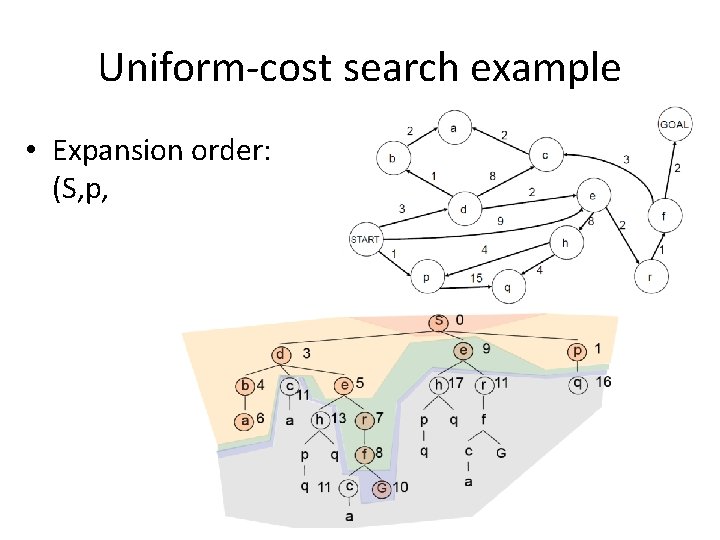
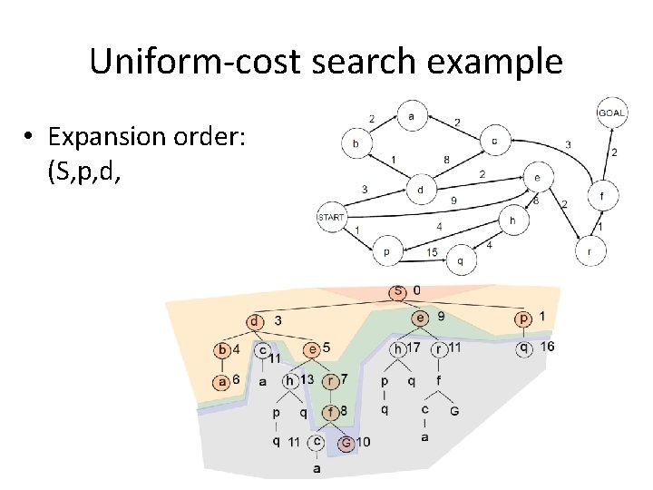
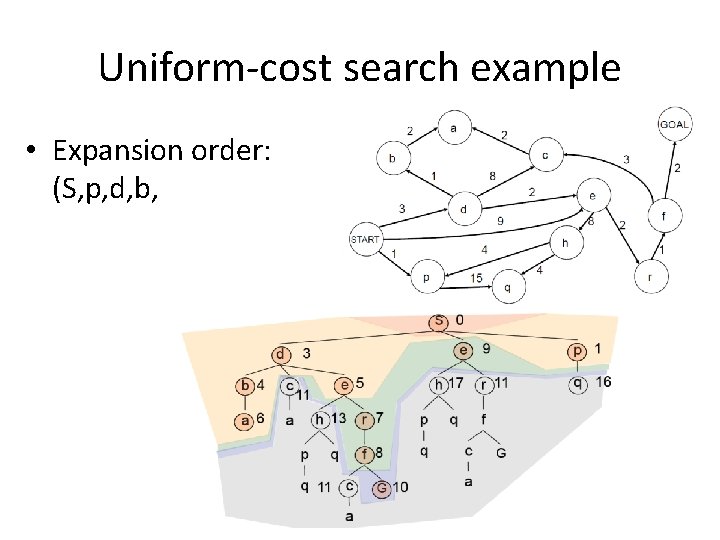
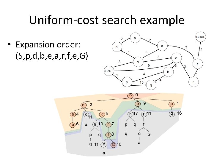
Uniform-cost search • For each frontier node, save the total cost of the path from the initial state to that node • Expand the frontier node with the lowest path cost • Implementation: frontier is a priority queue ordered by path cost • Equivalent to breadth-first if step costs all equal
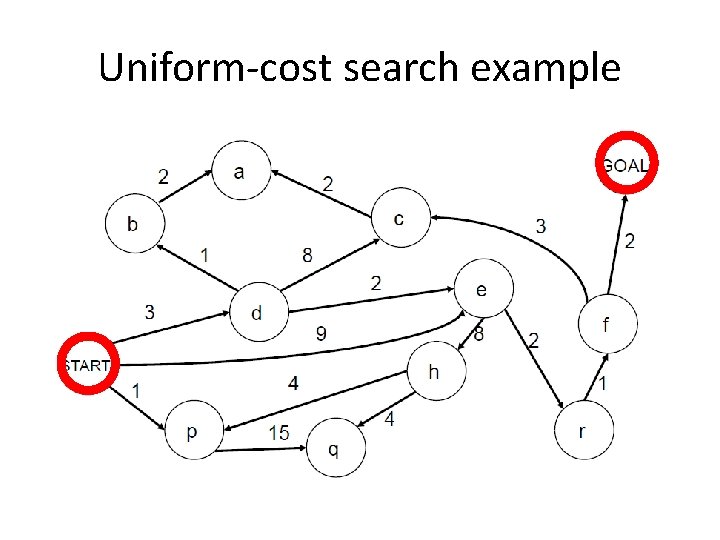
Uniform-cost search example
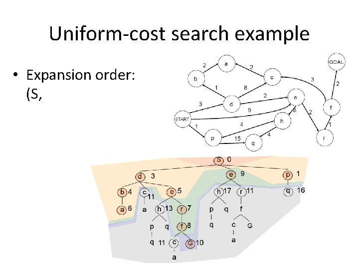
Uniform-cost search example • Expansion order: (S, p, d, b, e, a, r, f, e, G)
Uniform-cost search example • Expansion order: (S, p, d, b, e, a, r, f, e, G)
Uniform-cost search example • Expansion order: (S, p, d, b, e, a, r, f, e, G)
Uniform-cost search example • Expansion order: (S, p, d, b, e, a, r, f, e, G)
Uniform-cost search example • Expansion order: (S, p, d, b, e, a, r, f, e, G)
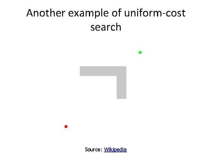
Another example of uniform-cost search Source: Wikipedia
Properties of uniform-cost search • Complete? Yes, if step costs are greater than some positive constant ε (gets stuck in infinite loop if there is a path with inifinite sequence of zero-cost actions) Optimal? Yes – nodes expanded in increasing order of path cost • Time? Number of nodes with path cost ≤ cost of optimal solution (C*), O(b. C*/ ε) This can be greater than O(bd): the search can explore long paths consisting of small steps before exploring shorter paths consisting of larger steps • Space? O(b. C*/ ε)
Informed search strategies • Idea: give the algorithm “hints” about the desirability of different states – Use an evaluation function to rank nodes and select the most promising one for expansion • Greedy best-first search • A* search
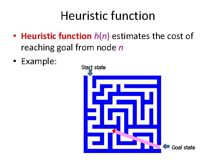
Heuristic function • Heuristic function h(n) estimates the cost of reaching goal from node n • Example: Start state Goal state
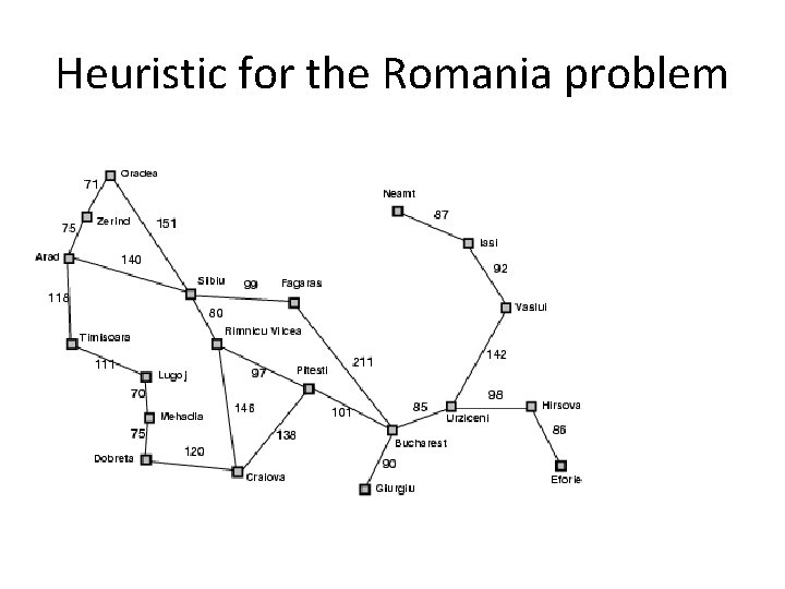
Heuristic for the Romania problem
Greedy best-first search • Expand the node that has the lowest value of the heuristic function h(n)
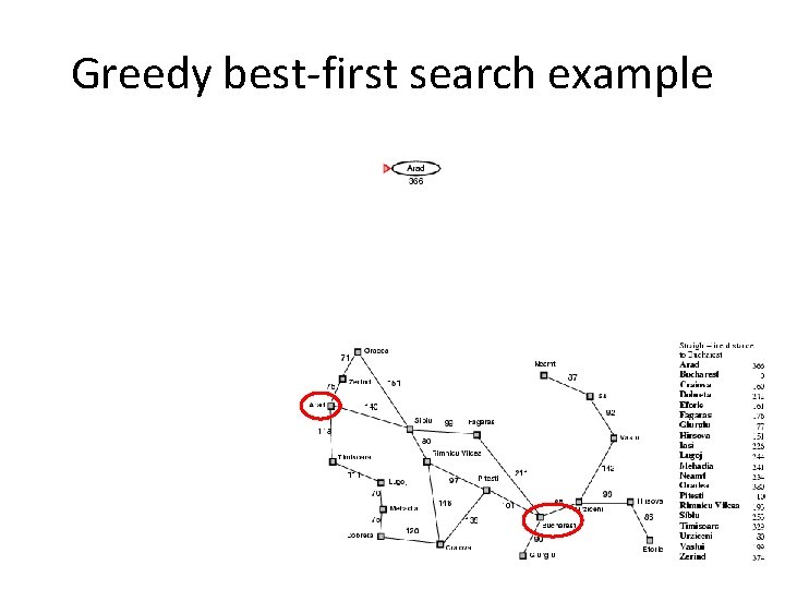
Greedy best-first search example
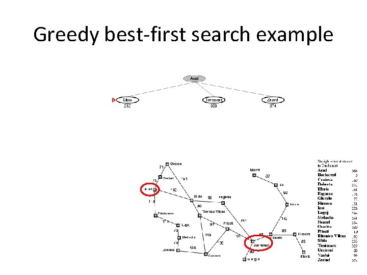
Greedy best-first search example
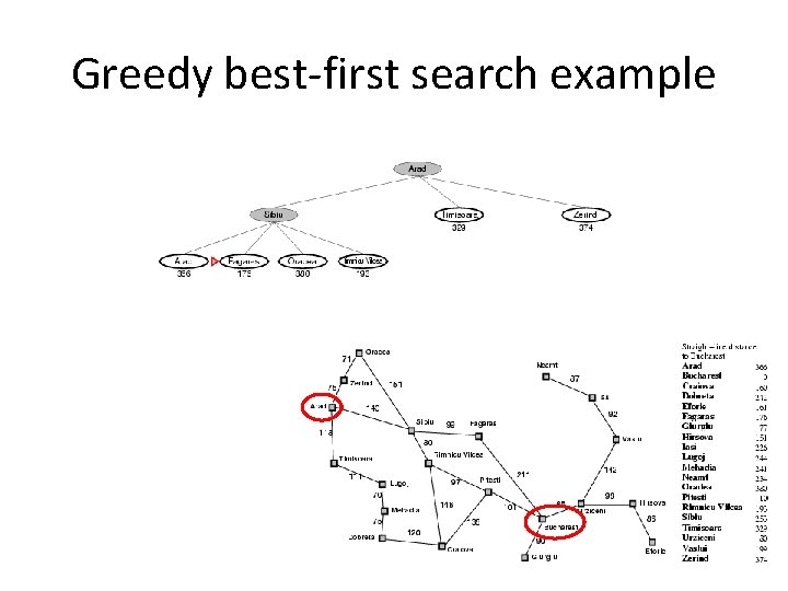
Greedy best-first search example
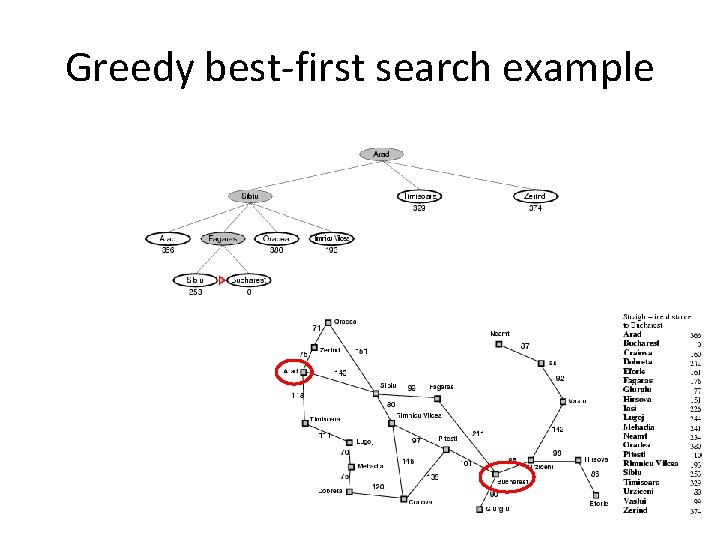
Greedy best-first search example
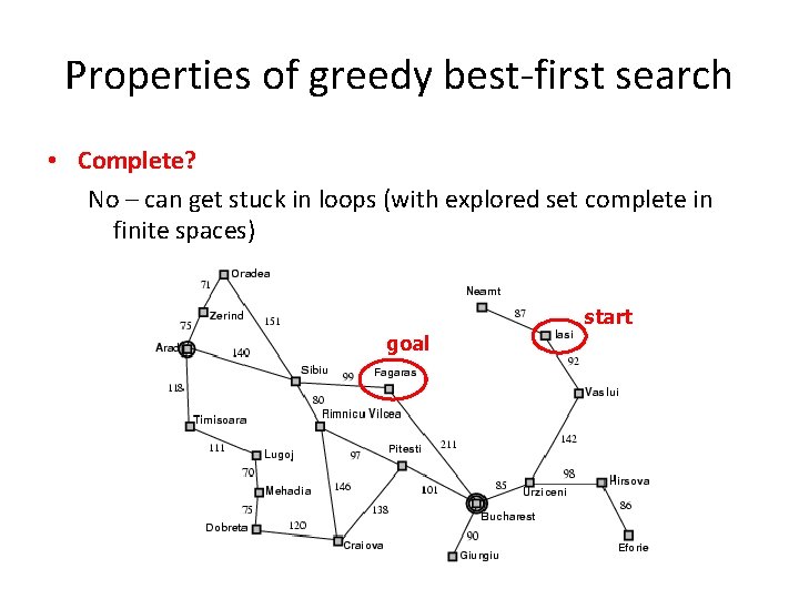
Properties of greedy best-first search • Complete? No – can get stuck in loops (with explored set complete in finite spaces) start goal
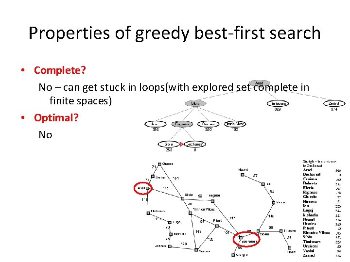
Properties of greedy best-first search • Complete? No – can get stuck in loops(with explored set complete in finite spaces) • Optimal? No
Properties of greedy best-first search • Complete? No – can get stuck in loops(with explored set complete in finite spaces) • Optimal? No • Time? • Space?
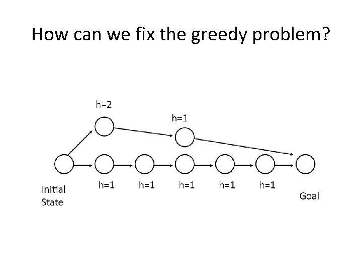
How can we fix the greedy problem?
Properties of greedy best-first search • Complete? No – can get stuck in loops(with explored set complete in finite spaces) • Optimal? No • Time? Worst case: O(bm) Can be much better with a good heuristic • Space? Worst case: O(bm)
A* search • Idea: avoid expanding paths that are already expensive • The evaluation function f(n) is the estimated total cost of the path through node n to the goal: f(n) = g(n) + h(n) g(n): cost so far to reach n (path cost) h(n): estimated cost from n to goal (heuristic)
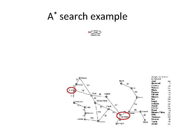
A* search example
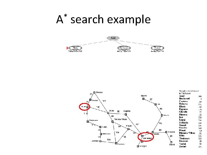
A* search example
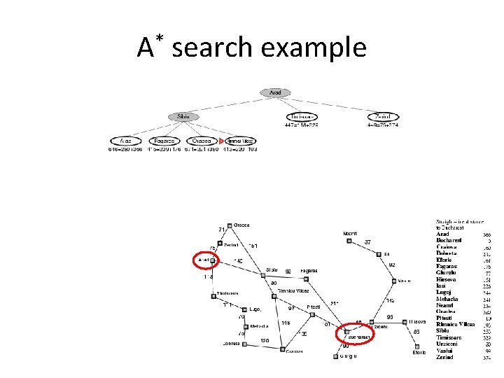
A* search example
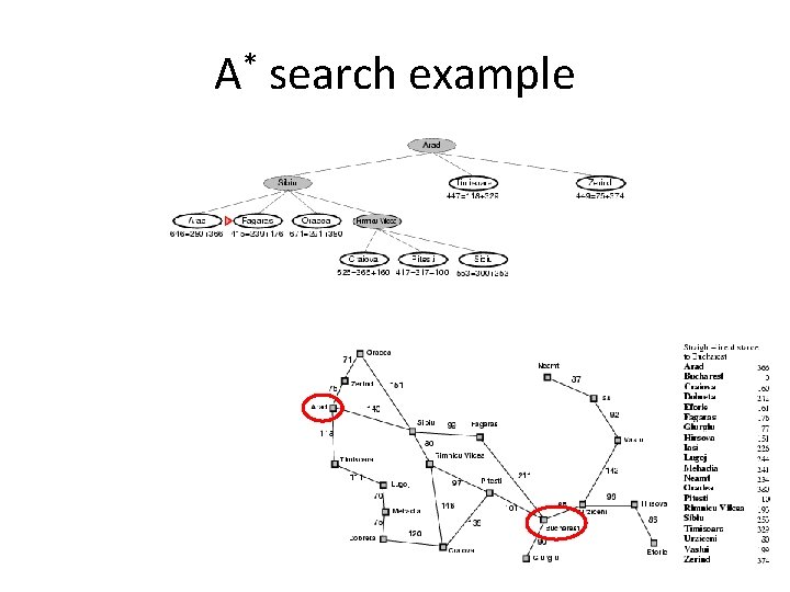
A* search example
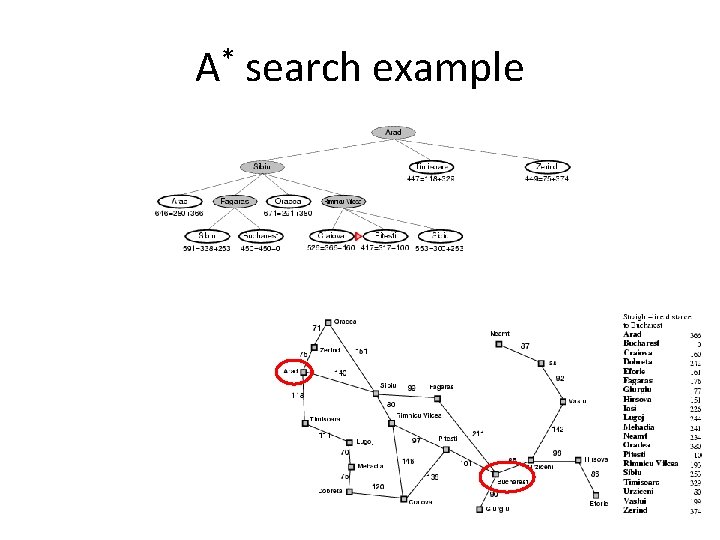
A* search example
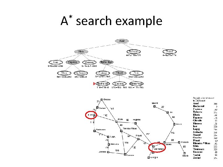
A* search example
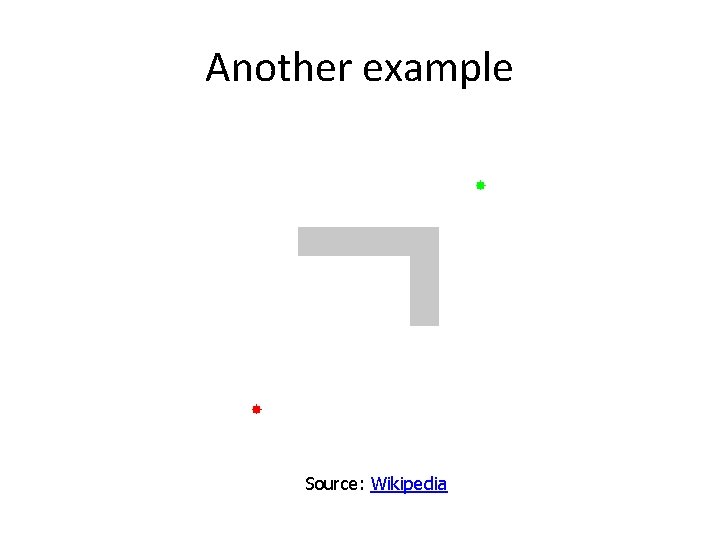
Another example Source: Wikipedia
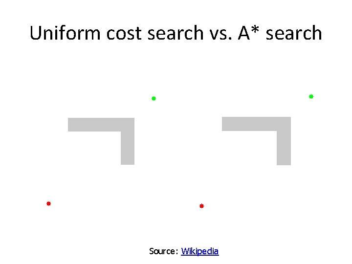
Uniform cost search vs. A* search Source: Wikipedia
Admissible heuristics • An admissible heuristic never overestimates the cost to reach the goal, i. e. , it is optimistic • A heuristic h(n) is admissible if for every node n, h(n) ≤ h*(n), where h*(n) is the true cost to reach the goal state from n • Is straight line distance admissible? – Yes, straight line distance never overestimates the actual road distance
Optimality of A* • Theorem: If h(n) is admissible, A* is optimal • Proof by contradiction: – Suppose A* terminates at goal state n with f(n) = g(n) = C but there exists another goal state n’ with g(n’) < C – Then there must exist a node n” on the frontier that is on the optimal path to n’ – Because h is admissible, we must have f(n”) ≤ g(n’) – But then, f(n”) < C, so n” should have been expanded first!
Properties of A* • Complete? Yes – unless there are infinitely many nodes with f(n) ≤ C* • Optimal? Yes • Time? Number of nodes for which g(n)+h(n) ≤ C* • Space? Number of nodes for which g(n)+h(n) ≤ C*
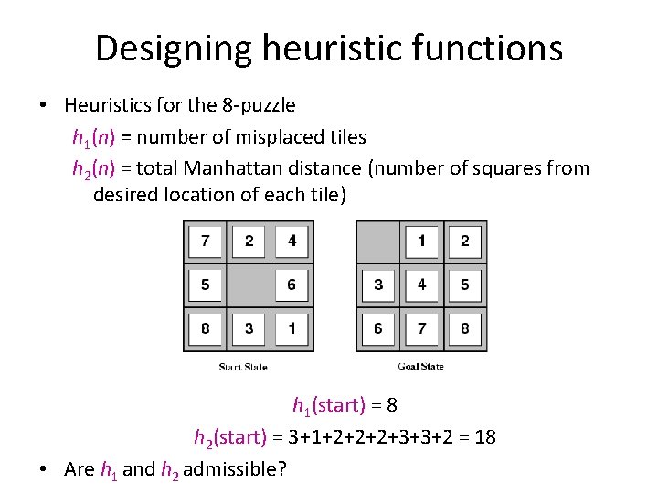
Designing heuristic functions • Heuristics for the 8 -puzzle h 1(n) = number of misplaced tiles h 2(n) = total Manhattan distance (number of squares from desired location of each tile) h 1(start) = 8 h 2(start) = 3+1+2+2+2+3+3+2 = 18 • Are h 1 and h 2 admissible?
Dominance • If h 1 and h 2 are both admissible heuristics and h 2(n) ≥ h 1(n) for all n, (both admissible) then h 2 dominates h 1 • Which one is better for search? – A* search expands every node with f(n) < C* or h(n) < C* – g(n) – Therefore, A* search with h 1 will expand more nodes
Dominance • Typical search costs for the 8 -puzzle (average number of nodes expanded for different solution depths): • d=12 IDS = 3, 644, 035 nodes A*(h 1) = 227 nodes A*(h 2) = 73 nodes • d=24 IDS ≈ 54, 000, 000 nodes A*(h 1) = 39, 135 nodes A*(h 2) = 1, 641 nodes
Heuristics from relaxed problems • A problem with fewer restrictions on the actions is called a relaxed problem • The cost of an optimal solution to a relaxed problem is an admissible heuristic for the original problem • If the rules of the 8 -puzzle are relaxed so that a tile can move anywhere, then h 1(n) gives the shortest solution • If the rules are relaxed so that a tile can move to any adjacent square, then h 2(n) gives the shortest solution
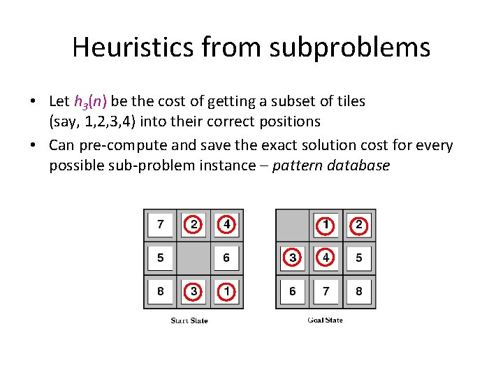
Heuristics from subproblems • Let h 3(n) be the cost of getting a subset of tiles (say, 1, 2, 3, 4) into their correct positions • Can pre-compute and save the exact solution cost for every possible sub-problem instance – pattern database
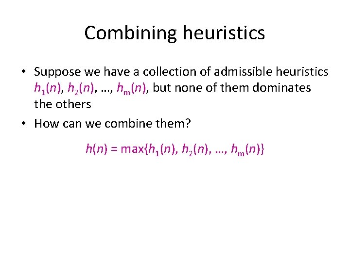
Combining heuristics • Suppose we have a collection of admissible heuristics h 1(n), h 2(n), …, hm(n), but none of them dominates the others • How can we combine them? h(n) = max{h 1(n), h 2(n), …, hm(n)}

A* Solving Tile Puzzle
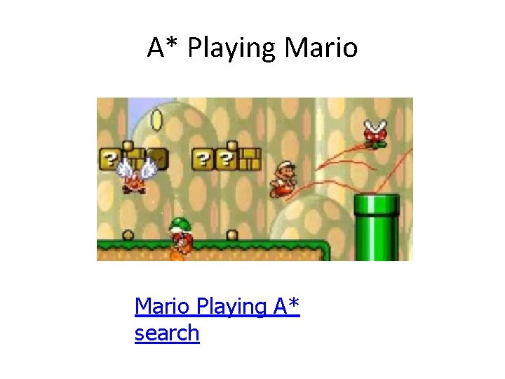
A* Playing Mario Playing A* search
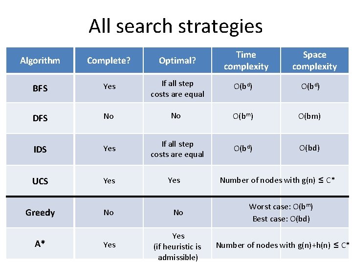
All search strategies Time complexity Space complexity Algorithm Complete? Optimal? BFS Yes If all step costs are equal O(bd) DFS No No O(bm) IDS Yes If all step costs are equal O(bd) UCS Yes Greedy A* Yes Number of nodes with g(n) ≤ C* No No Worst case: O(bm) Best case: O(bd) Yes (if heuristic is admissible) Number of nodes with g(n)+h(n) ≤ C*

Intro to CSPs
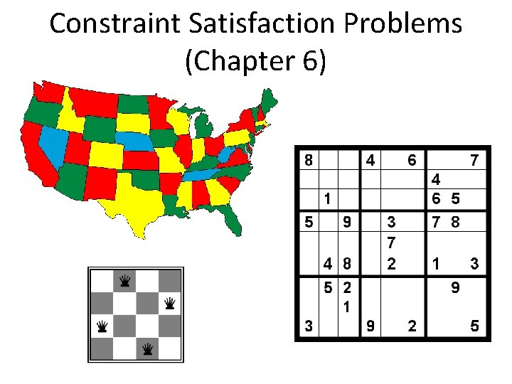
Constraint Satisfaction Problems (Chapter 6)
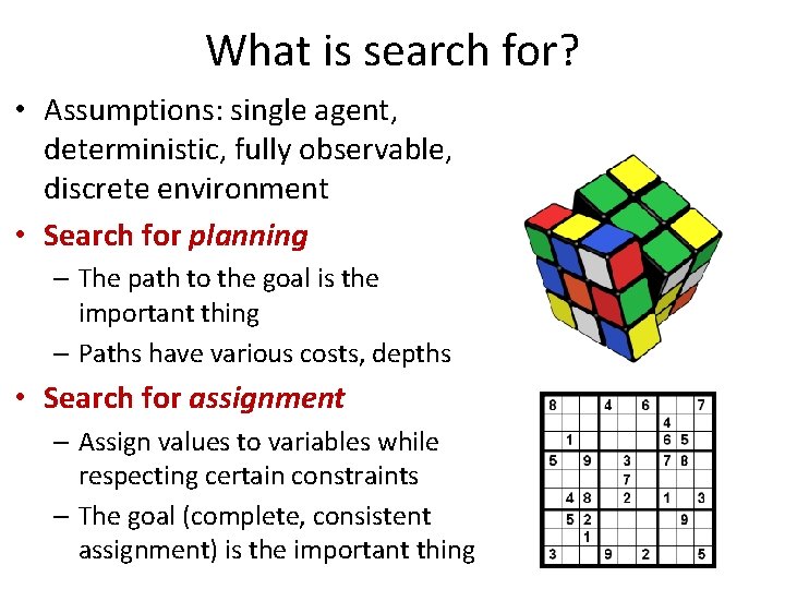
What is search for? • Assumptions: single agent, deterministic, fully observable, discrete environment • Search for planning – The path to the goal is the important thing – Paths have various costs, depths • Search for assignment – Assign values to variables while respecting certain constraints – The goal (complete, consistent assignment) is the important thing
Constraint satisfaction problems (CSPs) • Definition: – Xi is a set of variables {X 1 , … Xn} – Di is a set of domains {D 1 , . . . Dn} one for each variable – C is a set of constraints that specify allowable combinations of values – Solution is a complete, consistent assignment
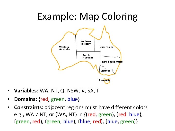
Example: Map Coloring • Variables: WA, NT, Q, NSW, V, SA, T • Domains: {red, green, blue} • Constraints: adjacent regions must have different colors e. g. , WA ≠ NT, or (WA, NT) in {(red, green), (red, blue), (green, red), (green, blue), (blue, red), (blue, green)}
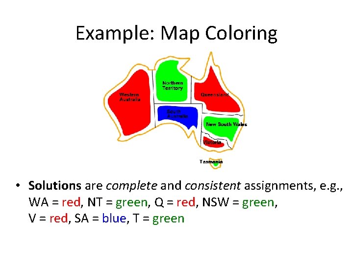
Example: Map Coloring • Solutions are complete and consistent assignments, e. g. , WA = red, NT = green, Q = red, NSW = green, V = red, SA = blue, T = green
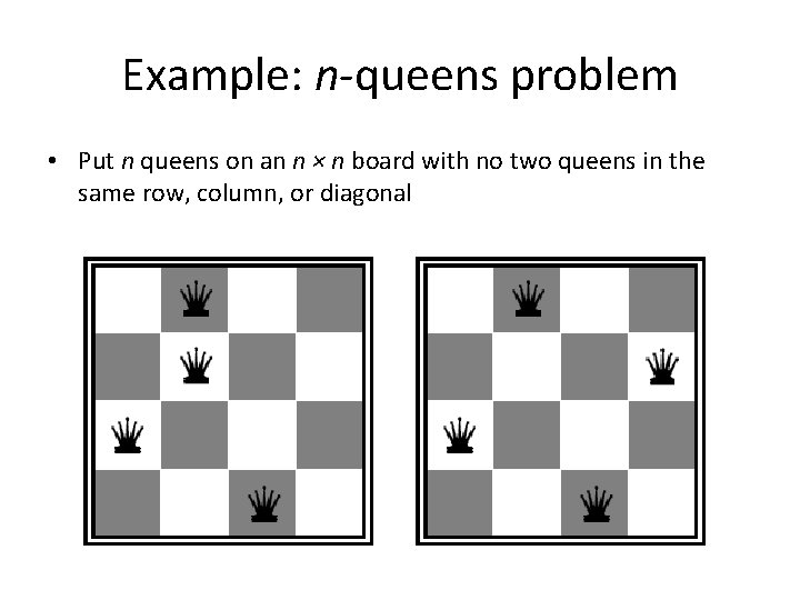
Example: n-queens problem • Put n queens on an n × n board with no two queens in the same row, column, or diagonal
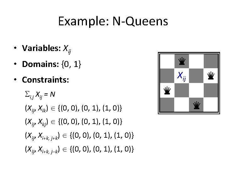
Example: N-Queens • Variables: Xij • Domains: {0, 1} • Constraints: i, j Xij = N (Xij, Xik) {(0, 0), (0, 1), (1, 0)} (Xij, Xkj) {(0, 0), (0, 1), (1, 0)} (Xij, Xi+k, j+k) {(0, 0), (0, 1), (1, 0)} (Xij, Xi+k, j–k) {(0, 0), (0, 1), (1, 0)} Xij
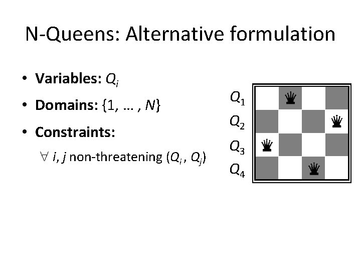
N-Queens: Alternative formulation • Variables: Qi • Domains: {1, … , N} • Constraints: i, j non-threatening (Qi , Qj) Q 1 Q 2 Q 3 Q 4
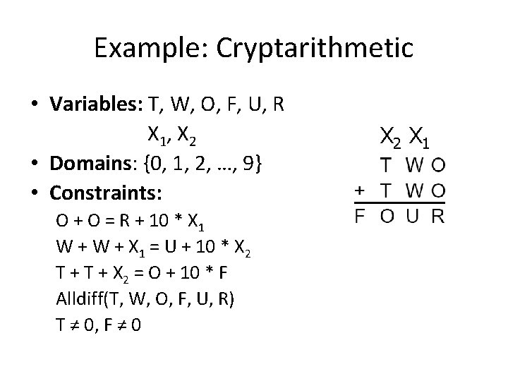
Example: Cryptarithmetic • Variables: T, W, O, F, U, R X 1 , X 2 • Domains: {0, 1, 2, …, 9} • Constraints: O + O = R + 10 * X 1 W + X 1 = U + 10 * X 2 T + X 2 = O + 10 * F Alldiff(T, W, O, F, U, R) T ≠ 0, F ≠ 0 X 2 X 1
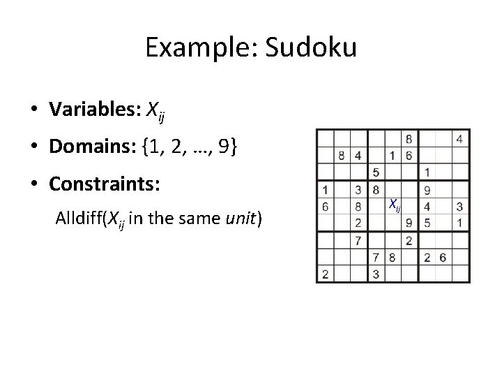
Example: Sudoku • Variables: Xij • Domains: {1, 2, …, 9} • Constraints: Alldiff(Xij in the same unit) Xij
- Slides: 70