SDE Statistics Mini Course SDE Closed form solution

SDE & Statistics Mini. Course SDE & Closed form solution: B&S model review Università di Verona, 2015 may 6 th Michele Bonollo michele. bonollo@imtlucca. it

Agenda • The problem • The B&S model • The call option formula • The call / put parity. No arbitrage concepts • The hedging issue • An actual spreadsheet implementation

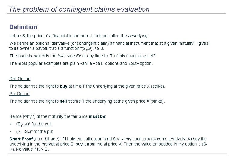
The problem of contingent claims evaluation Definition Let be St the price of a financial instrument. Is will be called the underlying. We define an optional derivative (or contingent claim) a financial instrument that at a given maturity T gives to its owner a payoff, trat is a function f(St, Q), f ≥ 0. The issue is: which is the fair value FV at any time t < T of this financial asset? The most popular examples are plain vanilla «call» options and «put» option. Call Option The holder has the right to buy at time T the underlying at the given price K (strike). Put Option. The holder has the right to sell at time T the underlying at the given price K (strike). Hence (why? ) at the maturity the fair price must be: • (ST- K)+ for the call • (K – ST)+ for the put Short Proof (no arbitrage). If I hold the call option, and S > K, my counterparty can alterntively: A) buy the underlying in the market at price S; buy it from me at price K. Then the value embedded in my option is (SK). No value if K > S.

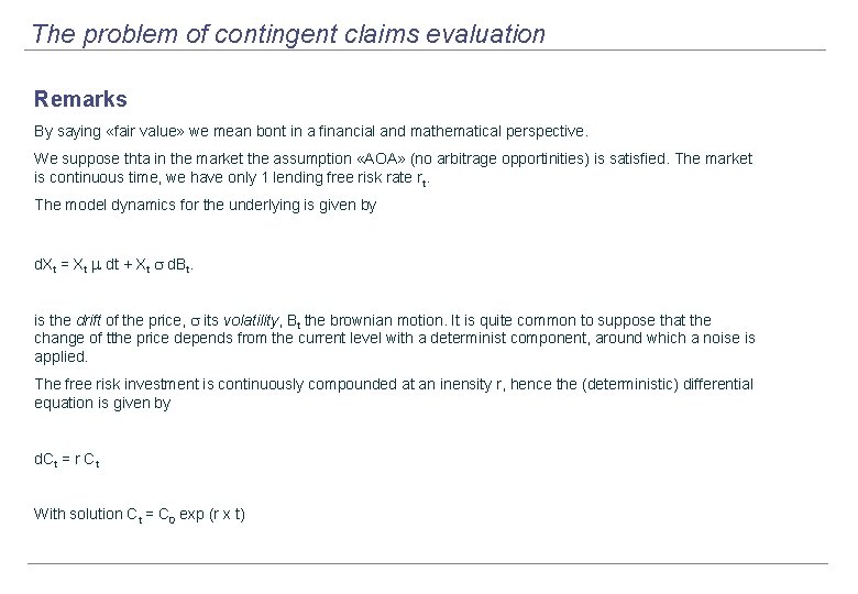
The problem of contingent claims evaluation Remarks By saying «fair value» we mean bont in a financial and mathematical perspective. We suppose thta in the market the assumption «AOA» (no arbitrage opportinities) is satisfied. The market is continuous time, we have only 1 lending free risk rate rt. The model dynamics for the underlying is given by d. Xt = Xt m dt + Xt s d. Bt. is the drift of the price, s its volatility, Bt the brownian motion. It is quite common to suppose that the change of tthe price depends from the current level with a determinist component, around which a noise is applied. The free risk investment is continuously compounded at an inensity r, hence the (deterministic) differential equation is given by d. Ct = r Ct With solution Ct = C 0 exp (r x t)

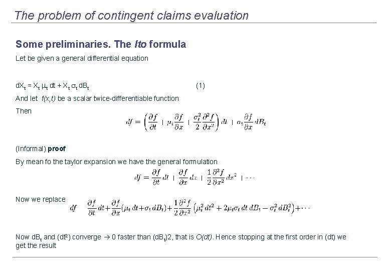
The problem of contingent claims evaluation Some preliminaries. The Ito formula Let be given a general differential equation d. Xt = Xt mt dt + Xt st d. Bt (1) And let f(x, t) be a scalar twice-differentiable function Then (Informal) proof By mean fo the taylor expansion we have the general formulation Now we replace with Xt and d. Xt Now d. Bt and (dt 2) converge 0 faster than (d. Bt)2, that is O(dt). Hence stopping at the first order in (dt) we get the result

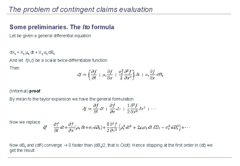
The problem of contingent claims evaluation Some preliminaries. The Ito formula Let be given a general differential equation d. Xt = Xt mt dt + Xt st d. Bt And let f(x, t) be a scalar twice-differntiable function Then (Informal) proof. By mean fo the taylor expansion we have the general formulation Now we replace with Xt and d. Xt Now d. Bt and (dt 2) converge 0 faster than (d. Bt)2, that is O(dt). Hence stopping at the first order in (dt) we get the result

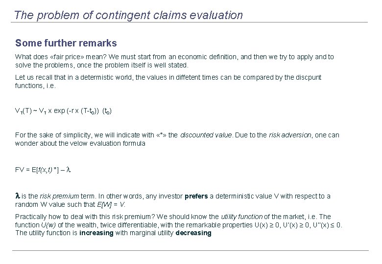
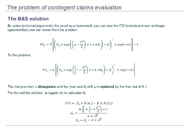
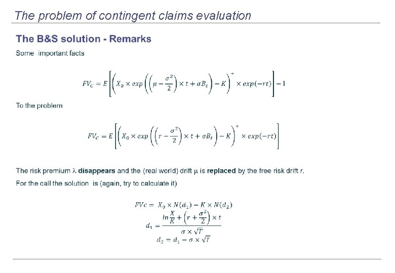
The problem of contingent claims evaluation Some further remarks What does «fair price» mean? We must start from an economic definition, and then we try to apply and to solve the problems, once the problem itself is well stated. Let us recall that in a determistic world, the values in diffetent times can be compared by the discpunt functions, i. e. VT(T) ~ VT x exp (-r x (T-t 0)) (t 0) For the sake of simplicity, we will indicate with «*» the discounted value. Due to the risk adversion, one can wonder about the velow evaluation formula FV = E[f(x, t) *] – l l is the risk premium term. In other words, any investor prefers a deterministic value V with respect to a random W value such that E[W] = V. Practically how to deal with this risk premium? We should know the utility function of the market, i. e. The function U(w) of the wealth, twice differentiable, with the remarkable properties U(x) ≥ 0, U’’(x) ≤ 0. The utility function is increasing with marginal utility decreasing

The problem of contingent claims evaluation

The problem of contingent claims evaluation

The problem of contingent claims evaluation

The problem of contingent claims evaluation

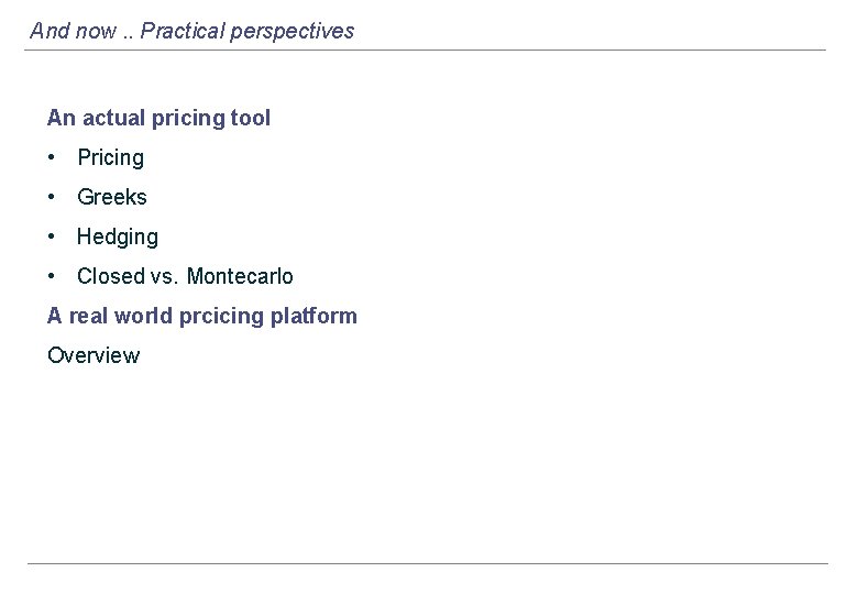
And now. . Practical perspectives An actual pricing tool • Pricing • Greeks • Hedging • Closed vs. Montecarlo A real world prcicing platform Overview