Screening the Data Tedious but essential Missing Data

Screening the Data Tedious but essential!

Missing Data • Missing Not at Random (MNAR) • Missing at Random (MAR) • Missing Completely at Random (MCAR)

Missing Not at Random (MNAR) • Are missing cases on Y • Missingness is related to the value of Y • Faculty salaries – those with high salaries may be reluctant to reveal them • Estimates of mean Y will be biased if use just the available data

Missing at Random (MAR) • Missingness on Y not related to value of Y • Or is related but through other variables on which we have data. • Faculty salary related to rank. • Higher rank = higher salary • If missingness is random within each rank, within-rank estimates will be unbiased. • Overall mean = weighted sum of withinrank estimates

Missing Completely at Random (MCAR) • There is no variable, observed or not, that is related to missingness of Y. • Ideal, not likely ever absolutely true.

Finding Patterns of Missingness • There is specialized software. You do not have it. • Can use SAS. • Can use SPSS with home license code. • Create missingness dummy variable • 0 = not missing, 1 = missing • Relate missingness to other variables.

Dealing with MCAR Data • Delete Cases: Will create no bias, but will lower power and precision. • Mean Substitution: For each missing value, substitute the group mean on that value. No bias for means, but will reduce standard deviations.

Dealing with MCAR Data • Regression: For each missing score, develop a multiple regression to predict score from other variables. Impute that predicted score. Regression towards mean will reduce variability.

Dealing with MAR Data • Deletion of Variables: If another variable can serve as a proxy. • Multiple Imputation – specialized software, may eliminate bias – Involves resampling techniques to generate several sets of predictions of missing scores – Analyze each set and then average the results across sets.

Dealing with MNAR Data • Sophisticated methods may reduce, but not eliminate, bias. • Pairwise Correlation Matrix – use as input to multivariate procedures. Different correlations will be based on different subsets of the data. Can produce very strange results, not recommended.

Missing Item Data Within Unidimensional Scale • Assume each item measures the same construct. • For each subject, compute the means on the items which do have data. • Set to missing the scale scores for subjects who have answered fewer than a threshold number of items. • This procedure is known as “Person Mean Imputation. ”

Identifying Outliers • Univariate: Box and whiskers plots • Multivariate: Compute Mahalanobis Distance or Leverage. Investigate cases with high values. Use outlier dummy variable to compare outliers with inliers. • Regression Diagnostics: o Leverage: Cases with unusual values on the predictor variables

Outliers o Standardized Residuals: Cases whose actual Y is far from predicted Y. o Cook’s D: Cases with values that make them have great influence on the regression solution.

Dealing with Outliers • Investigate: May be bad data. May be able to correct the data, may not. May represent cases not properly considered part of the population of interest. • Out-of-Range Values: Even if not outliers, these are bad data that need correction.

Dealing with Outliers • Set to Missing: If all else fails. • Delete the Case: For example, if convinced the respondent was not even reading the questions. – “I frequently visit planets outside of our solar system. ” – “I make all of my own clothes. ”

Dealing with Outliers • Transform the Variable: If outliers are valid but contributing to skewness. • Change the Score: For example, reduce very high score to a value a small bit higher than the remaining highest score. See Howell’s discussion of “Winsorizing. ”

Assumptions of the Analysis • Check Outliers First: Dealing with outliers may resolve the problems below. • Normality: Look at plots and measures of skewness and kurtosis. Ignore tests of significance, like Kolgomorov-Smirnov. May need to use different analysis. • Homogeneity of Variance: Does the variance differ considerably across groups? May need to transform or use different analysis.

Assumptions of the Analysis • Homoscedasticity: Carefully inspect the residuals. May need to transform data or use a different analysis. • Homogeneity of Variance/Covariance Matrices (across groups): Box’s M. • Sphericity: For univariate-approach related samples ANOVA. Check with Mauchley’s Test. Correct the df or use a multivariate approach instead.

Assumptions of the Analysis • Homogeneity of Regression: In ANCOV, we assume the relationship between Y and the predictors is constant across groups. Test the Groups x Predictor(s) interactions. • Linear Relationships: Look at plots. If necessary, transform variables or use curvilinear techniques.

Multicollinearity • One predictor is nearly perfectly correlated with the other predictors. • Makes the regression coefficients unstable across random samples from the same population. • Makes complicated the interpretation of unique effects.

Detecting Multicollinearity • For each predictor, compute the R 2 between it and the other predictors. If very high (. 9 or more), there is a problem. • SAS will compute tolerance = (1 – that R 2 ). If very low, there is a problem. • If R 2 = 1, the correlation matrix is singular, cannot be inverted, the analysis crashes – Predictors = Verbal SAT, Math SAT, Total SAT.

Variance Inflation Factor • VIF = 1/tolerance. If high, there is a problem. • How High? • Some say 10, some say 5, a few say 2. 5. • If R 2 =. 9, tolerance =. 1, VIF = 10.

Dealing with Multicollinearity • Drop a Predictor – may resolve the problem. • Combine Predictors – into a composite variable • Principle Components Analysis – conduct the analysis on the resulting weighed linear combinations of the variables. Can then transform the results back to the original variables.

SAS 1 • Look at the command lines in the SAS program. • Always give every case a unique ID number, so you can locate it later. • Label variables if their SAS name is not informative. • input ID 1 -3 @5 (Q 1 -Q 138) (1. ); label Q 1='Sex' Q 3 = 'Age';

SAS 2 • Recode values that represent missing data. • On several variables, such as “number of biological brothers, ” response 5 was “do not know. ” • if Q 15 = 5 then Q 15 =. ; if Q 16 = 5 then q 16 =. ;

SAS 3 & 4 • Transform variable to reduce positive skewness • age_sr = sqrt(Q 3); age_log = log 10(Q 3); age_inv = -1/(Q 3); • Dichotomize variable – transformation of last resort. • if q 3 = 1 then age_di = 1; else if q 3 > 1 then age_di = 2;

SAS 5 & 6 • Create composite variable for number of brothers + number of sisters. • SIBS = Q 15 + Q 16; • Transform to reduce positive skewness • sibs_sr = sqrt(sibs); sibs_log = log 10(sibs); sibs_in = -1/sibs;

SAS 7 • Create mental variable and associated missingness variable. • Father’s mental health + Mother’s + Siblings’ • MENTAL = Q 62 + Q 65 + Q 67; Mental. Miss = 0; If Mental=. then Mental. Miss = 1;

SAS 8 • Transform to reduce negative skewness • Mental 2 = Mental*Mental; Mental 3 = Mental**3; Ment_exp = EXP(Mental); R_Ment = 13 - Mental; R_Ment_sr = sqrt(R_Ment); R_Ment_log = log 10(R_Ment);

SAS 9 • Dichotomize Mental • if 0 LE Mental LE 9 then Ment_di=1; else if Mental > 9 then Ment_di=2; • Be careful – SAS codes missing data with an extreme negative number.

Dichot Not ! • It has been common practice to dichotomize badly skewed variables. • Irwin & Mc. Clelland (2003) have demonstrated that this is poor practice • Dichotomizing Continuous Variables -- a bad idea

SAS 10 • Check for missing data and out-of-range values. • proc means min max n nmiss; var q 1 -q 10 q 50 -q 70; run; • OUTPUT DOCUMENT

SAS 11 • Check for skewness & kurtosis • proc means min max n nmiss skewness kurtosis; var Q 3 age_sr -- Mental 2 -- R_Ment_log; run; • OUTPUT DOCUMENT

SAS 12 • Check distributions of variables with few values • proc freq; tables q 3 age_di sibs mental ment_di; run; • OUTPUT DOCUMENT

SAS 13 • Locate cases with bad data • data duh; set delmel; if q 9 > 3; proc print; var q 9; id id; run; • Case 159 has out-of-range on item Q 9. • OUTPUT DOCUMENT

SAS 14 • Check correlates of missingness. • proc corr nosimple data=delmel; var Mental. Miss; with Q 1 Q 3 Q 5 Q 6 sibs; run; • Mental. Miss negatively correlated with sibs. • Duh, some subjects have missing data(doesn’t apply) on number of brothers or number of sisters. • Instead of Mental = Q 62+Q 65+Q 67, use Mental = Mean(of Q 62 Q 65 Q 67);

Multidimensional Outliers • investigate observations with leverage greater than 2 p/n, “where n is the number of observations used to fit the model, and p is the number of parameters in the model. ” • 4 variables: Q 1 Q 3 Q 6 mental + intercept • 193 observations • 2*5/193 =. 052

SAS 15 • Identify multivariate outliers • proc reg data=delmel; model id = Q 1 Q 3 Q 6 mental; output out=hat H=Leverage; run; data outliers; set hat; if leverage >. 052;

SAS 15 • Identify multivariate outliers • proc print; var id Q 1 Q 3 Q 6 mental leverage; run; proc means mean; var Q 1 Q 3 Q 6 mental; run; • As a group, the outliers are older than the overall sample. • All three students aged 25 or older are included among the outliers.

Survey Scoundrels • These sloths do not even read the questions, they just answer randomly to get whatever incentive is available for completing the survey. • My daughter’s shock upon discovering this. • Monitor how long it takes respondents to complete the survey.

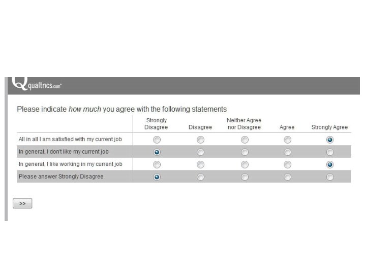
Items to Help Detect Scoundrels • Repeat same item, compare responses • “I frequently visit with aliens from other planets. ” • “I make all of my own clothes. ”

Code Booking • Variable names (should be descriptive) • What the variable really is (with survey data, what was the question asked) • For discrete variables, what were the response options and how were they coded. • SAS: Use variable labels and value formats. • SPSS: Use variable labels and value labels