Scot Farm A linear programming farm level model

Scot. Farm A linear programming farm level model for Scottish farms Shailesh Shrestha Bouda Vosough Ahmadi Steven Thomson Andrew Barnes Leading the way in Agriculture and Rural Research, Education and Consulting

Background • Farm. Adapt – 2000 – CAP Agenda 2000, adaptations, market prices, nutrient balance • FDLP – 2002 – Climate change impact on English dairy farms • Teagasc. Mod – 2004 – CAP MTR, Milk quota Removal, Climate change 2

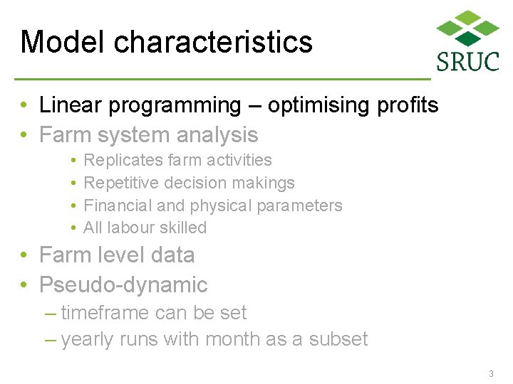
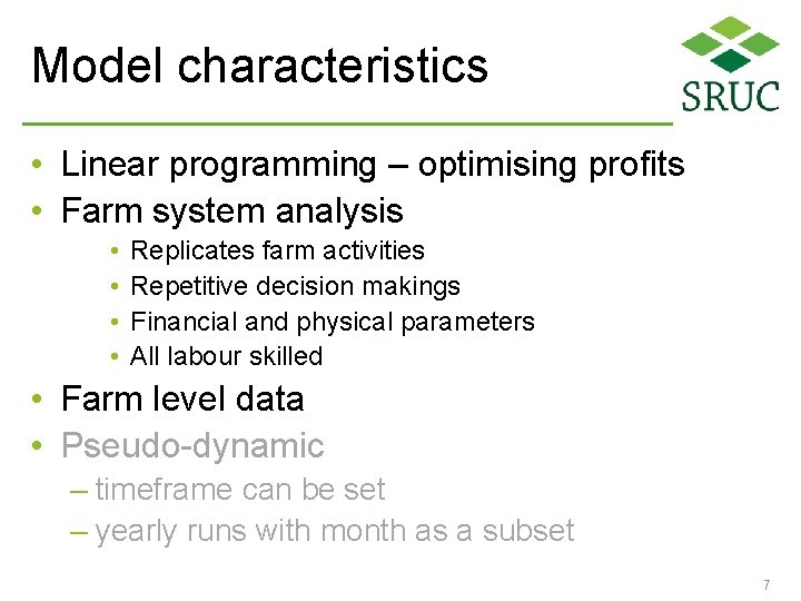
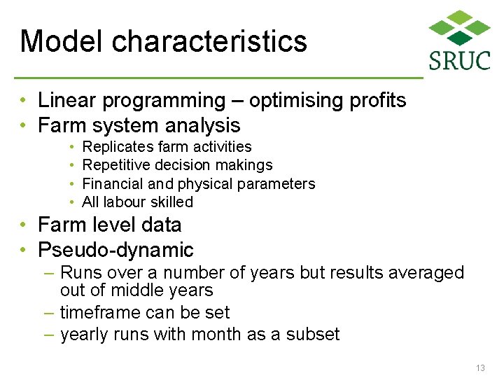
Model characteristics • Linear programming – optimising profits • Farm system analysis • • Replicates farm activities Repetitive decision makings Financial and physical parameters All labour skilled • Farm level data • Pseudo-dynamic – timeframe can be set – yearly runs with month as a subset 3

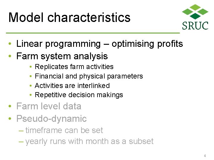
Model characteristics • Linear programming – optimising profits • Farm system analysis • • Replicates farm activities Financial and physical parameters Activities are interlinked Repetitive decision makings • Farm level data • Pseudo-dynamic – timeframe can be set – yearly runs with month as a subset 4

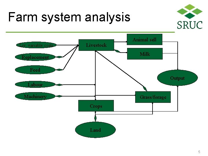
Farm system analysis Liv. variable costs Livestock Animal sell Milk Replacement Feed Output Labour Machinery Grass/forage Crops Land 5

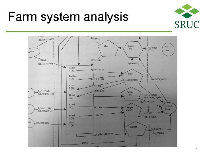
Farm system analysis 6

Model characteristics • Linear programming – optimising profits • Farm system analysis • • Replicates farm activities Repetitive decision makings Financial and physical parameters All labour skilled • Farm level data • Pseudo-dynamic – timeframe can be set – yearly runs with month as a subset 7

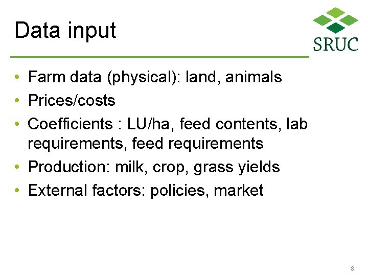
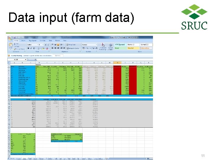
Data input • Farm data (physical): land, animals • Prices/costs • Coefficients : LU/ha, feed contents, lab requirements, feed requirements • Production: milk, crop, grass yields • External factors: policies, market 8

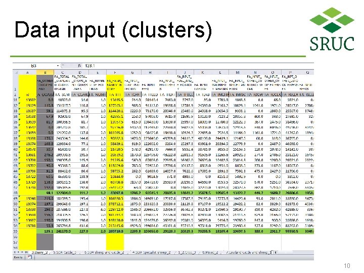
Data input (FAS) • Scottish Farm Accountancy Survey (FAS) – Around 480 farms – Contains physical/ financial data • Cluster analysis – System, production, size, milk yield, labour, farm margins, feed, costs – Farm groups identified – Representative farms 9

Data input (clusters) 10

Data input (farm data) 11

Data input (feed) 12

Model characteristics • Linear programming – optimising profits • Farm system analysis • • Replicates farm activities Repetitive decision makings Financial and physical parameters All labour skilled • Farm level data • Pseudo-dynamic – Runs over a number of years but results averaged out of middle years – timeframe can be set – yearly runs with month as a subset 13

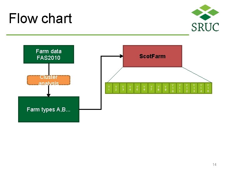
Flow chart Farm data FAS 2010 Cluster analysis Scot. Farm Y 1 Y 2 Y 3 Y 4 Y 5 Y 6 Y 7 Y 8 Y 9 Y 1 0 Y 1 1 Y 1 2 Y 1 3 Y 1 4 Y 1 5 Farm types A, B. . . 14

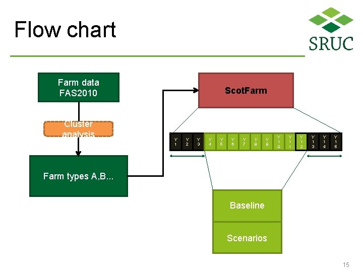
Flow chart Farm data FAS 2010 Cluster analysis Scot. Farm Y 1 Y 2 Y 3 Y 4 Y 5 Y 6 Y 7 Y 8 Y 9 Y 1 0 Y 1 1 Y 1 2 Y 1 3 Y 1 4 Y 1 5 Farm types A, B. . . Baseline Scenarios 15

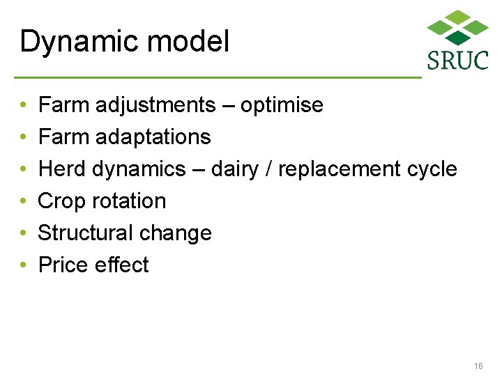
Dynamic model • • • Farm adjustments – optimise Farm adaptations Herd dynamics – dairy / replacement cycle Crop rotation Structural change Price effect 16

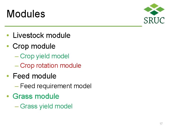
Modules • Livestock module • Crop module – Crop yield model – Crop rotation module • Feed module – Feed requirement model • Grass module – Grass yield model 17

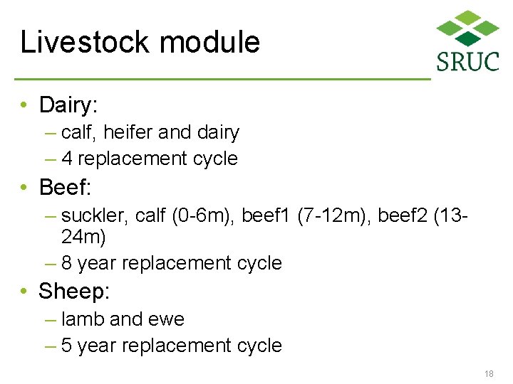
Livestock module • Dairy: – calf, heifer and dairy – 4 replacement cycle • Beef: – suckler, calf (0 -6 m), beef 1 (7 -12 m), beef 2 (1324 m) – 8 year replacement cycle • Sheep: – lamb and ewe – 5 year replacement cycle 18

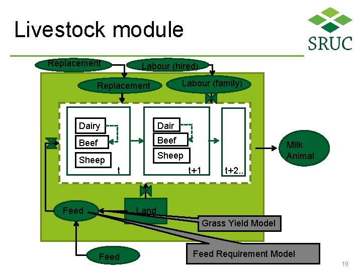
Livestock module Replacement Labour (hired) Labour (family) Replacement Beef Dair y. Beef Sheep Dairy t Milk Animal t+1 t+2. . . t Feed Land Grass Yield Model Feed Requirement Model 19

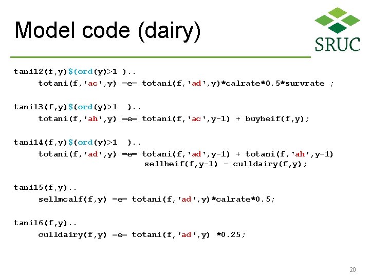
Model code (dairy) tani 12(f, y)$(ord(y)>1 ). . totani(f, 'ac', y) =e= totani(f, 'ad', y)*calrate*0. 5*survrate ; tani 13(f, y)$(ord(y)>1 ). . totani(f, 'ah', y) =e= totani(f, 'ac', y-1) + buyheif(f, y); tani 14(f, y)$(ord(y)>1 ). . totani(f, 'ad', y) =e= totani(f, 'ad', y-1) + totani(f, 'ah', y-1) sellheif(f, y-1) - culldairy(f, y); tani 15(f, y). . sellmcalf(f, y) =e= totani(f, 'ad', y)*calrate*0. 5; tani 16(f, y). . culldairy(f, y) =e= totani(f, 'ad', y) *0. 25; 20

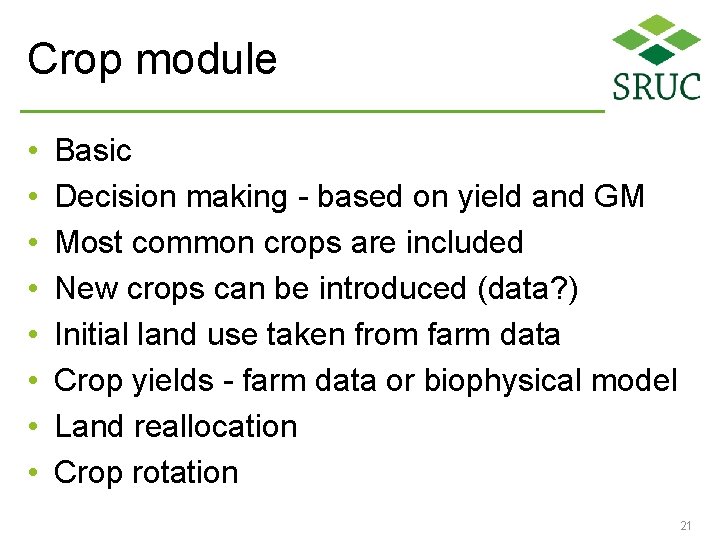
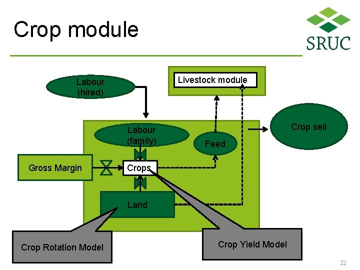
Crop module • • Basic Decision making - based on yield and GM Most common crops are included New crops can be introduced (data? ) Initial land use taken from farm data Crop yields - farm data or biophysical model Land reallocation Crop rotation 21

Crop module Livestock module Labour (hired) Labour (family) Gross Margin Crop sell Feed Crops Land Crop Rotation Model Crop Yield Model 22

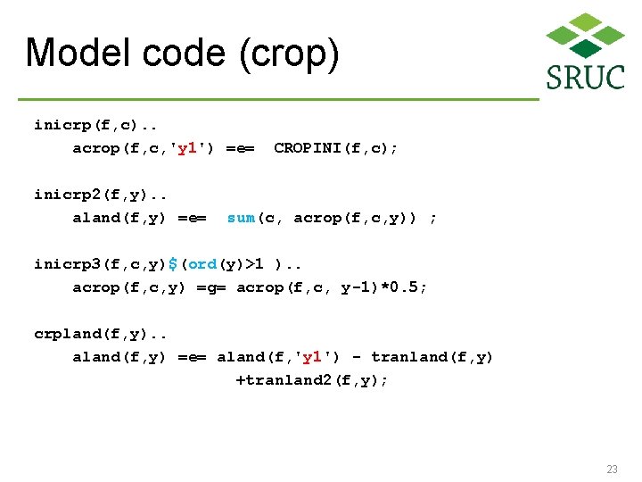
Model code (crop) inicrp(f, c). . acrop(f, c, 'y 1') =e= inicrp 2(f, y). . aland(f, y) =e= CROPINI(f, c); sum(c, acrop(f, c, y)) ; inicrp 3(f, c, y)$(ord(y)>1 ). . acrop(f, c, y) =g= acrop(f, c, y-1)*0. 5; crpland(f, y). . aland(f, y) =e= aland(f, 'y 1') - tranland(f, y) +tranland 2(f, y); 23

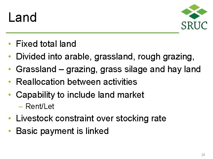
Land • • • Fixed total land Divided into arable, grassland, rough grazing, Grassland – grazing, grass silage and hay land Reallocation between activities Capability to include land market – Rent/Let • Livestock constraint over stocking rate • Basic payment is linked 24

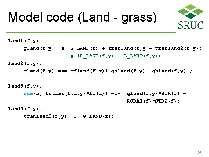
Model code (Land - grass) land 1(f, y). . gland(f, y) =e= G_LAND(f) + tranland(f, y)- tranland 2(f, y); # +R_LAND(f, y) - L_LAND(f, y); land 2(f, y). . gland(f, y) =e= gfland(f, y)+ gsland(f, y)+ ghland(f, y) ; land 3(f, y). . sum(a, totani(f, a, y)*LU(a)) =l= gland(f, y)*STR(f) + RGRAZ(f)*STR 2(f); land 4(f, y). . tranland 2(f, y) =l= G_LAND(f); 25

Feed module • Feed considered – Fresh grass, grass silage, hay, maize silage whole crop grain, concentrate • Feed – produced on farm/bought in • Energy and protein content required for each feed 26

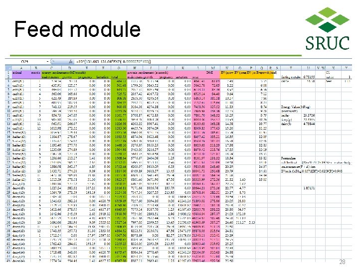
Feed requirement model • Model is written in excel • Based on feed requirement criteria set by Alderman and Cottrill (1993) • Determines monthly requirement of energy, protein and feed intake per animal • Considers species, age, production level of an individual animal 27

Feed module 28

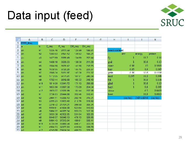
Data input (feed) 29

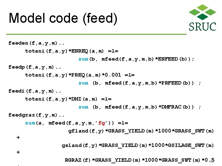
Model code (feed) feeden(f, a, y, m). . totani(f, a, y)*ENREQ(a, m) =l= sum(b, mfeed(f, a, y, m, b)*ENFEED(b)); feedp(f, a, y, m). . totani(f, a, y)*PREQ(a, m)*0. 001 =l= sum (b, mfeed(f, a, y, m, b)*PRFEED(b)) ; feedi(f, a, y, m). . totani(f, a, y)*DMI(a, m) =l= sum (b, mfeed(f, a, y, m, b)*DMFRAC(b)) ; feedgraz(f, y, m). . sum(a, mfeed(f, a, y, m, ’fg’)) =l= gfland(f, y)*GRASS_YIELD(m)*1000*GRASS_SWT(m) + gsland(f, y)*GRASS_YIELD(m)*1000*GSILAGE_SWT(m) + RGRAZ(f)*GRASS_YIELD(m)*1000*GRASS_SWT(m)*0. 5 30

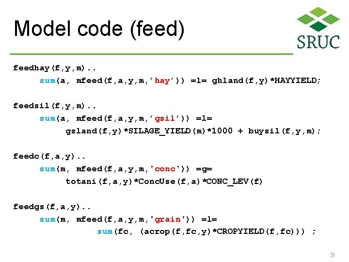
Model code (feed) feedhay(f, y, m). . sum(a, mfeed(f, a, y, m, ’hay’)) =l= ghland(f, y)*HAYYIELD; feedsil(f, y, m). . sum(a, mfeed(f, a, y, m, ’gsil’)) =l= gsland(f, y)*SILAGE_YIELD(m)*1000 + buysil(f, y, m); feedc(f, a, y). . sum(m, mfeed(f, a, y, m, 'conc')) =g= totani(f, a, y)*Conc. Use(f, a)*CONC_LEV(f) feedgs(f, a, y). . sum(m, mfeed(f, a, y, m, 'grain')) =l= sum(fc, (acrop(f, fc, y)*CROPYIELD(f, fc))) ; 31

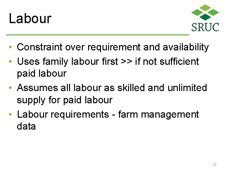
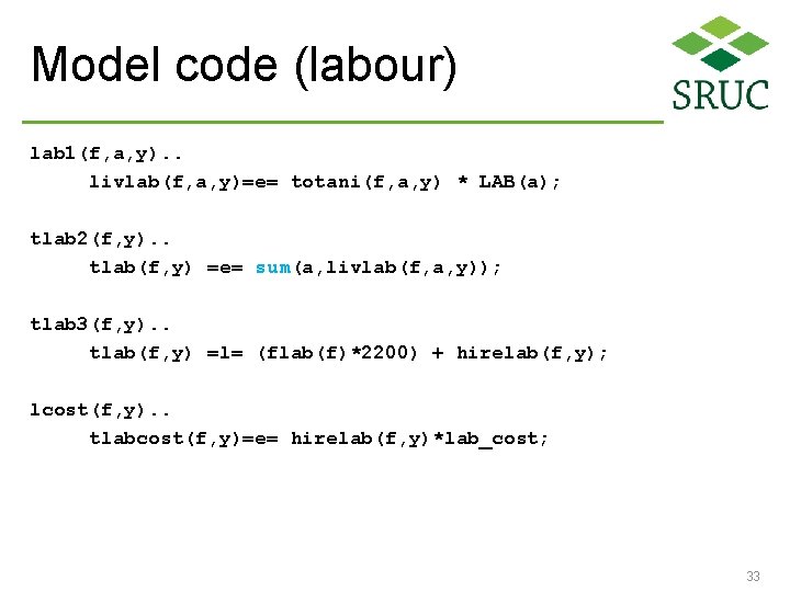
Labour • Constraint over requirement and availability • Uses family labour first >> if not sufficient paid labour • Assumes all labour as skilled and unlimited supply for paid labour • Labour requirements - farm management data 32

Model code (labour) lab 1(f, a, y). . livlab(f, a, y)=e= totani(f, a, y) * LAB(a); tlab 2(f, y). . tlab(f, y) =e= sum(a, livlab(f, a, y)); tlab 3(f, y). . tlab(f, y) =l= (flab(f)*2200) + hirelab(f, y); lcost(f, y). . tlabcost(f, y)=e= hirelab(f, y)*lab_cost; 33

Subsidy payments • • Included in the objective function BPS is linked with the total farm land LFAS is added as a parameter for each farm Under CAP reform scenarios, different rates of payments can be linked to different land use 34

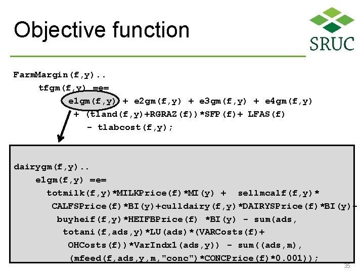
Objective function Farm. Margin(f, y). . tfgm(f, y) =e= e 1 gm(f, y) + e 2 gm(f, y) + e 3 gm(f, y) + e 4 gm(f, y) + (tland(f, y)+RGRAZ(f))*SFP(f)+ LFAS(f) - tlabcost(f, y); dairygm(f, y). . e 1 gm(f, y) =e= totmilk(f, y)*MILKPrice(f)*MI(y) + sellmcalf(f, y)* CALFSPrice(f)*BI(y)+culldairy(f, y)*DAIRYSPrice(f)*BI(y)buyheif(f, y)*HEIFBPrice(f) *BI(y) - sum(ads, totani(f, ads, y)*LU(ads)*(VARCosts(f)+ OHCosts(f))*Var. Indx 1(ads, y)) - sum((ads, m), (mfeed(f, ads, y, m, "conc")*CONCPrice(f)*0. 001)); 35

Subsidy payments • • Included in the objective function BPS is linked with the total farm land LFAS is added as a parameter for each farm Under CAP reform scenarios, different rates of payments can be linked to different land use 36

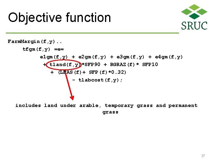
Objective function Farm. Margin(f, y). . tfgm(f, y) =e= e 1 gm(f, y) + e 2 gm(f, y) + e 3 gm(f, y) + e 4 gm(f, y) + tland(f, y)*SFP 90 + RGRAZ(f)* SFP 10 + (LFAS(f)+ SFP(f)*0. 32) - tlabcost(f, y); includes land under arable, temporary grass and permanent grass 37

Outputs • • Farm margins Land use Animal numbers Feed use Production level Costs of production Marginal costs 38

Applications • Policy impacts: CAP reforms and Milk quota removal • Climate change impacts • Farmers adaptations • Structural change • Cost analysis: GHG mitigation options • Capable of running individual farms or representative farms 39

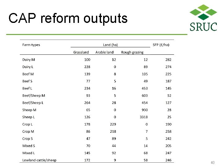
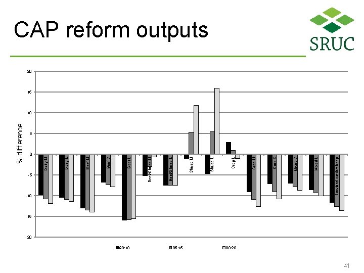
CAP reform outputs 40

-5 90: 10 85: 15 Mixed L Mixed S Crop S Lowland cattle/sheep -10 Crop M Crop L Sheep M Beef/Sheep L Beef/Sheep M Beef L Beef S Beef M Dairy L Dairy M CAP reform outputs 20 15 10 5 0 -15 -20 80: 20 41

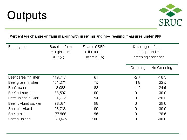
Outputs Percentage change on farm margin with greening and no-greening measures under SFP Farm types Beef cereal finisher Beef grass finisher Beef rearer Beef hill suckler Beef upland sukler Beef lowland suckler Sheep lowland Sheep hill Sheep upland Baseline farm margins inc SFP (£) 119, 747 121, 271 113, 583 86, 507 64, 772 96, 031 93, 763 77, 966 79, 475 Share of SFP in the farm margin (%) 61 75 83 100 94 98 100 95 100 % change in farm margin under greening scenarios Greening No Greening -2. 7 -1. 8 -1. 2 0 0 0 -18. 5 -22. 5 -24. 9 -30. 0 -28. 3 -29. 0 -30. 0 -28. 5 -30. 0

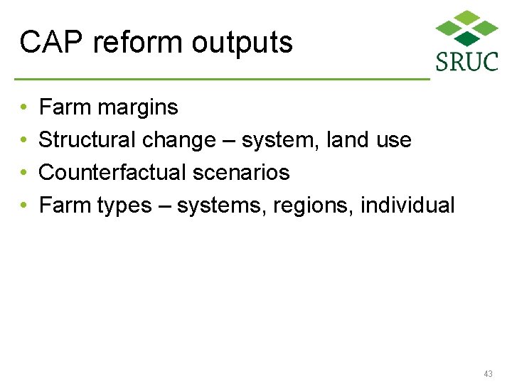
CAP reform outputs • • Farm margins Structural change – system, land use Counterfactual scenarios Farm types – systems, regions, individual 43

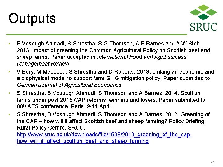
Outputs • • B Vosough Ahmadi, S Shrestha, S G Thomson, A P Barnes and A W Stott, 2013. Impact of greening the Common Agricultural Policy on Scottish beef and sheep farms. Paper accepted in International Food and Agribusiness Management Review V Eory, M Mac. Leod, S Shrestha and D Roberts, 2013. Linking an economic and a biophysical model to support farm GHG mitigation policy. Paper submitted to German Journal of Agricultural Economics S Shrestha, B Vosough Ahmadi, S Thomson and A Barnes, 2014. Scottish farms under post 2015 CAP reforms: winners and losers. Paper submitted to 88 th AES conference, Paris, 9 -11 April. S Shrestha, B Vosough Ahmadi, S Thomson and A Barnes, 2013. Greening of the CAP – how will it affect Scottish beef and sheep farming? Policy Briefing, Rural Policy Centre, SRUC. http: //www. sruc. ac. uk/downloads/file/1538/2013_greening_of_the_caphow_will_it_affect_scottish_beef_and_sheep_farming 44

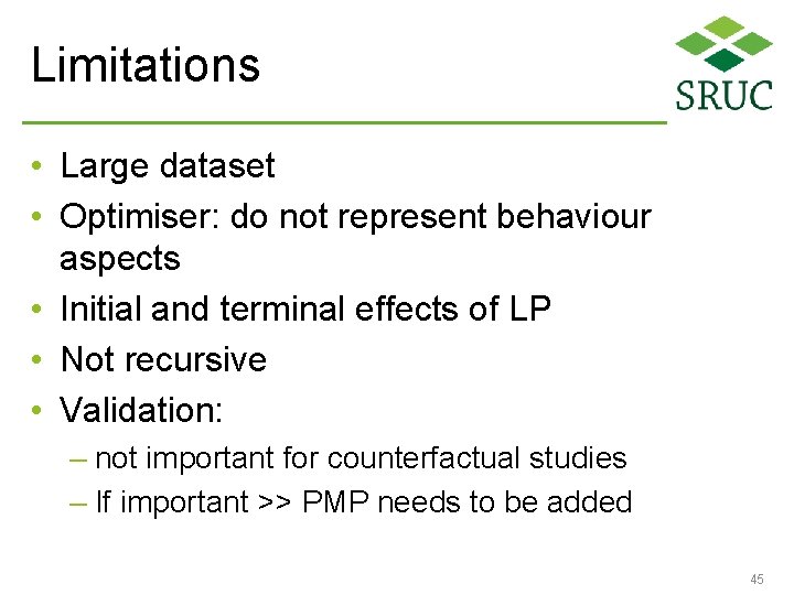
Limitations • Large dataset • Optimiser: do not represent behaviour aspects • Initial and terminal effects of LP • Not recursive • Validation: – not important for counterfactual studies – If important >> PMP needs to be added 45

Leading the way in Agriculture and Rural Research, Education and Consulting