scipy interpolate 1 d interp 1 d 1


 • • 线性 1 d插值 (interp 1 d) 1 d样条插值 (interpolate. spl.")


 A, k, theta = 10, 1.")
")


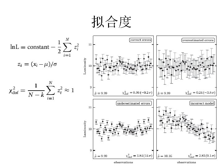
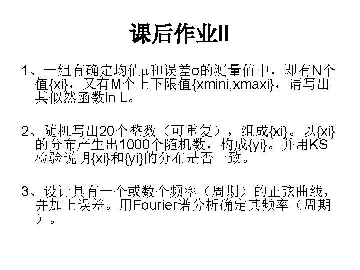
 检验")

 https: //github. com/pymc-devs/pymc")


- Slides: 50
插值(scipy. interpolate) • • 线性 1 d插值 (interp 1 d) 1 d样条插值 (interpolate. spl. XXX) 2 d样条插值 (bisplrep) RBF(radial basis function)插值/平滑
import numpy as np from scipy. interpolate import Rbf import matplotlib. pyplot as plt from matplotlib import cm # 2 -d tests - setup scattered data x = np. random. rand(100)*4. 0 -2. 0 y = np. random. rand(100)*4. 0 -2. 0 z = x*np. exp(-x**2 -y**2) ti = np. linspace(-2. 0, 100) XI, YI = np. meshgrid(ti, ti) # use RBF rbf = Rbf(x, y, z, epsilon=2) ZI = rbf(XI, YI) # plot the result n = plt. Normalize(-2. , 2. ) plt. subplot(1, 1, 1) plt. pcolor(XI, YI, ZI, cmap=cm. jet) plt. scatter(x, y, 100, z, cmap=cm. jet) plt. title('RBF interpolation - multiquadrics') plt. xlim(-2, 2) plt. ylim(-2, 2) plt. colorbar() plt. show()
import numpy as np import scipy. linalg as splin import matplotlib. pyplot as plt c 1, c 2= 5. 0, 2. 0 i = np. r_[1: 11] xi = 0. 1*i yi = c 1*np. exp(-xi)+c 2*xi zi = yi + 0. 05*np. max(yi)*np. random. randn(len(yi)) A = np. c_[np. exp(-xi)[: , np. newaxis], xi[: , np. newaxis]] c, resid, rank, sigma = splin. lstsq(A, zi) print c, resid, rank, sigma xi 2 = np. r_[0. 1: 1. 0: 100 j] yi 2 = c[0]*np. exp(-xi 2) + c[1]*xi 2 plt. plot(xi, zi, 'x', xi 2, yi 2) plt. axis([0, 1. 1, 3. 0, 5. 5]) plt. xlabel('$x_i$') plt. title('Data fitting with linalg. lstsq') plt. show()
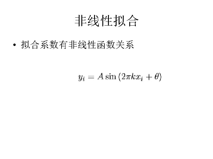
from numpy import x = arange(0, 6 e-2/30) A, k, theta = 10, 1. 0/3 e-2, pi/6 y_true = A*sin(2*pi*k*x+theta) y_meas = y_true + 2*random. randn(len(x)) def residuals(p, y, x): A, k, theta = p err = y-A*sin(2*pi*k*x+theta) return err def peval(x, p): return p[0]*sin(2*pi*p[1]*x+p[2]) p 0 = [8, 1/2. 3 e-2, pi/3] print array(p 0) # [ 8. 43. 4783 1. 0472] from scipy. optimize import leastsq plsq = leastsq(residuals, p 0, args=(y_meas, x)) print plsq[0] # [ 10. 9437 33. 3605 0. 5834] print array([A, k, theta]) # [ 10. 3333 0. 5236] import matplotlib. pyplot as plt. plot(x, peval(x, plsq[0]), x, y_meas, 'o', x, y_true) plt. title('Least-squares fit to noisy data') plt. legend(['Fit', 'Noisy', 'True']) plt. show()
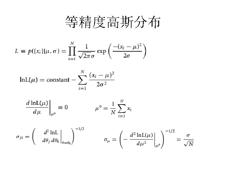
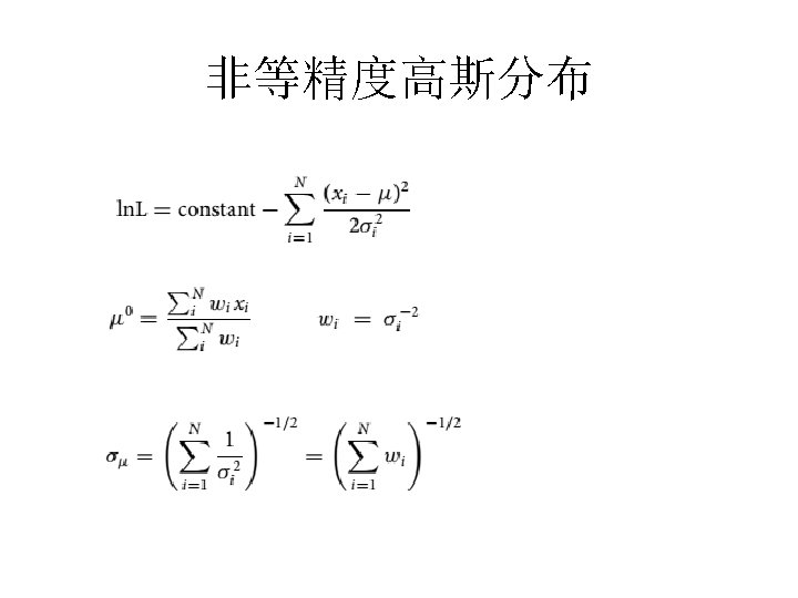
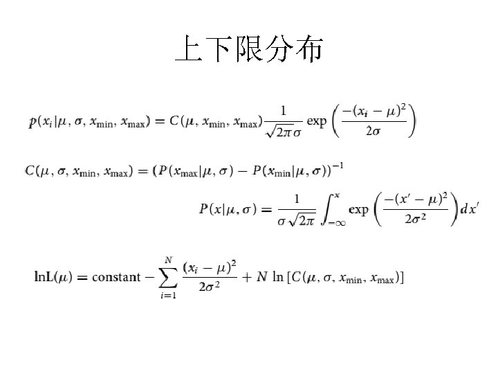
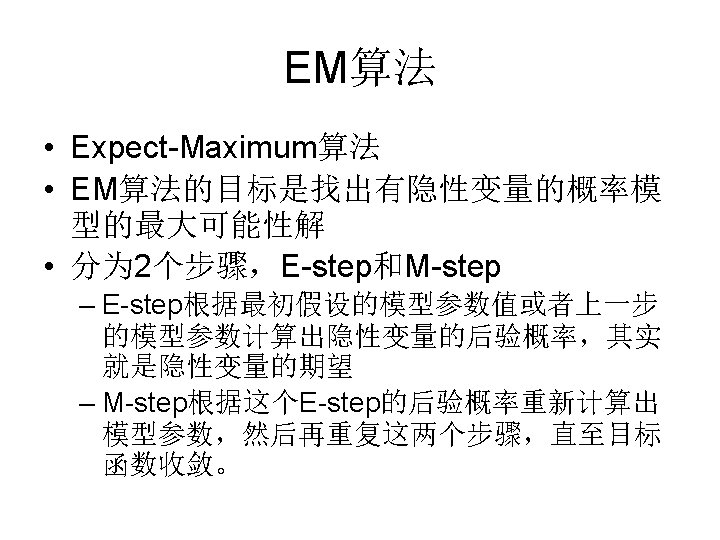
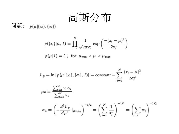
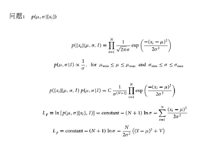
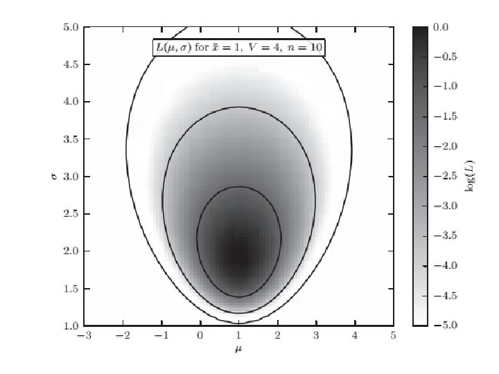
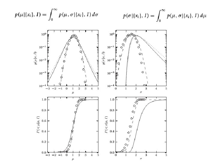
Maximum Likelihood Estimation (MLE)
求极值scipy. optimize A collection of general-purpose optimization routines. fmin -- Nelder-Mead Simplex algorithm (uses only function calls) fmin_powell -- Powell's (modified) level set method (uses only function calls) fmin_cg -- Non-linear (Polak-Ribiere) conjugate gradient algorithm (can use function and gradient). fmin_bfgs -- Quasi-Newton method (Broydon-Fletcher-Goldfarb-Shanno); (can use function and gradient) fmin_ncg -- Line-search Newton Conjugate Gradient (can use function, gradient and Hessian). leastsq -- Minimize the sum of squares of M equations in N unknowns given a starting estimate. Constrained Optimizers (multivariate) fmin_l_bfgs_b -- Zhu, Byrd, and Nocedal's L-BFGS-B constrained optimizer (if you use this please quote their papers -- see help) fmin_tnc -- Truncated Newton Code originally written by Stephen Nash and adapted to C by Jean-Sebastien Roy. fmin_cobyla -- Constrained Optimization BY Linear Approximation
Kolmogorov–Smirnov (K-S) 检验
高斯分布? • Anderson–Darling检验 • Shapiro–Wilk检验
Markov chain Monte Carlo (MCMC) https: //github. com/pymc-devs/pymc
Fourier变换scipy. fftpack
离散Fourier变换