SCILAB AND ITS APPLICATIONS By R K Singh

SCILAB AND IT’S APPLICATIONS By R. K Singh

1. ARITHMETIC OPERATION

1. Scilab as Calculator • Scilab is an inbuilt calculator. • It performs all simple and scientific calculations.

Example

2. Variable Assignment >> a=1 a= 1 For example let’s take b=2 >> b=2 b= 2 So we can easily calculate c=a+b >> c=a+b c= 3

Example

2. TRIGONOMETRIC OPERATION
 a = 1. --> b=cos(%pi/2) b = 6. 123")
3. Trigonometric Calculation --> a=sin(%pi/2) a = 1. --> b=cos(%pi/2) b = 6. 123 D-17 --> c=a+b c = 1. --> c=sin(%pi/2)+cos(%pi/2)

Example

3. MATRIX OPERATION

Creating Matrix

4. Creating a Matrix Example 1 : We want to create a 2*2 matrix with element [2 3; 4 5] then we will write >> a=[2 3; 4 5] a= 2. 4. 3. 5.

Example

5. Creating a Matrix Example 2 : We want to create a 2*3 matrix with element [2 3 4; 4 5 6] then we will write >> a=[2 3 4; 4 5 6] a= 2. 3. 4. 4. 5. 6.

Example

Matrix Arithmetic

6. Addition, Subtraction, Multiplication. . Example 3 : Create two matrices of 2*2 with elements a=[2 3; 4 5] and b= [3 5; 6 7] , add them and find the value of c=a+b. >> a=[2 3; 4 5] >> c=a+b a= 2. 3. 4. 5. >> b= [3 5; 6 7] b= 3. 5. 6. 7. c= 5. 8. 10. 12.

Example

Features of the Matrix

7. Transpose Example 4 : Find the transpose of matrix A= [4 2 5; 4 8 6; 7 8 7] >> A= [4 2 5; 4 8 6; 7 8 7] A= 4. 2. 5. 4. 8. 6. 7. 8. 7. >> B= A’ 4. 4. 7. 2. 8. 8. 5. 6. 7.

Example

8. Diagonal Element Example 5 : Find the diagonal of matrix A= [4 2 5; 4 8 6; 7 8 7] >> A= [4 2 5; 4 8 6; 7 8 7] A= 4. 2. 5. 4. 8. 6. 7. 8. 7. >> B=diag(A) B= 4. 8.

Example

9. Inverse Example 6 : Find the inverse of matrix A= [4 5 6; 7 8 9; 10 11 12] >> A= [4 5 6; 7 8 9; 10 11 18] A= 4. 5. 6. 7. 8. 9. 10. 11. 18. >> B=inv(A) B= -2. 5 1. 3333333 0. 1666667 2. -0. 6666667 -0. 3333333 0. 1666667

Example

10. Identity Matrix Example 7 : Create an identity matrix of 3*3 elements >> A= eye(3, 3) A= 1. 0. 0. 0. 1.

Example

11. Unit Matrix: Example 8 : Create an unit matrix of 3*3 elements >> A= ones(3, 3) A= 1. 1. 1.

Example

12. Determinant of a Matrix: : Example 9 : Calculate the determinant value of a matrix A= [4 5 6; 7 8 9; 10 11 12] àA= [4 5 6; 7 8 9; 10 11 18] 4. 5. 6. 7. 8. 9. 10. 11. 18. --> B=det(A) B = -18.

Example

3. Signal Plot

2 -D Plot

1 Steps : First create the range of the signal or plotting points. >> a=0: 0. 01: 1; 2 Steps : Create the function for the signal. >> b=sin(%pi*a); 3 Plotting : Plot the function for the signal. >> plot(a, b)

13. 2 D Plot Example 10 : Create a sine wave àa=0: 0. 01: 10; àb=sin(2*%pi*a); àplot(a, b)

Example

Result
; àplot(a, b) àxlabel('X Axis') àylabel('Y")
14. Title, Label, Legend àa=0: 0. 01: 1; àb=sin(2*%pi*a); àplot(a, b) àxlabel('X Axis') àylabel('Y Axis') àtitle(‘SIN Wave’) àlegend(‘SIN Wave’)

Example

Result

2 -D Multiple Image Figure Plot

15. 2 D Subplot 1. Step: First create the program for sine function. a=0: 0. 01: 1; b=sin(2*%pi*a); plot(a, b) xlabel('X Axis') ylabel('Y Axis') title(‘Sin’)
;")
2. Step : Write the program for cos wave. a=0: 0. 01: 1; b=cos(2*%pi*a); plot(a, b) xlabel('X Axis') ylabel('Y Axis') title(‘Cos’)
; c=cos(2*%pi*a); figure(1) plot(a,")
3. Step : Combine the codes. a=0: 0. 01: 1; b=sin(2*%pi*a); c=cos(2*%pi*a); figure(1) plot(a, b) xlabel('X Axis') ylabel('Y Axis') figure(2) plot(a, c) xlabel('X Axis') ylabel('Y Axis')

Result

2 -D Multiple Image Figure Subplot

16. 2 D Subplot 1. Step: First create the program for sine function. a=0: 0. 01: 1; b=sin(2*%pi*a); plot(a, b) xlabel('X Axis') ylabel('Y Axis')
;")
2. Step : Write the program for cos wave. a=0: 0. 01: 1; b=cos(2*%pi*a); plot(a, b) xlabel('X Axis') ylabel('Y Axis') title(‘Cos’)
; c=cos(2*%pi*a); subplot(1, 2,")
3. Step : Combine the codes. a=0: 0. 01: 1; b=sin(2*%pi*a); c=cos(2*%pi*a); subplot(1, 2, 1) plot(a, b) xlabel('X Axis') ylabel('Y Axis') subplot(1, 2, 2) plot(a, c) xlabel('X Axis') ylabel('Y Axis')

Result

3 -D Plot

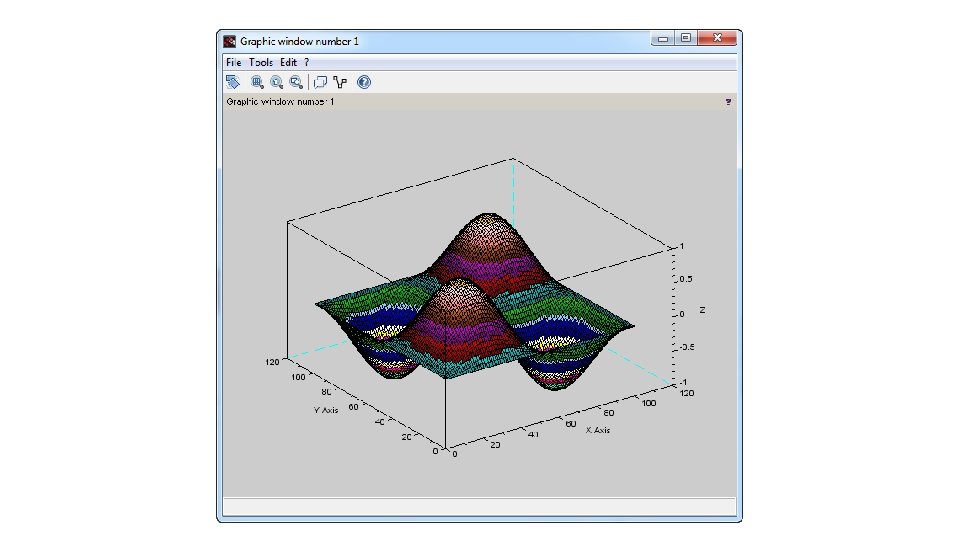
1. 1 Steps : First create the range of the signal or plotting points. >> a=0: 0. 01: 1; 1. 2 Steps : Create the function for the signal. >> b=sin(2*%pi*a); 1. 3 Step : Create third dimension. >> c=b’*b; 1. 4 Steps : Surface Plot >> surf(c)
; àc=b’*b; àsurf(c)")
17. 3 D Plot àa=0: 0. 01: 1; àb=sin(2*%pi*a); àc=b’*b; àsurf(c)

Example

Result
; àc=b’*b; àsurf(c) àxlabel('X Axis') àylabel('Y")
14. Title, Label, Legend àa=0: 0. 01: 1; àb=sin(2*%pi*a); àc=b’*b; àsurf(c) àxlabel('X Axis') àylabel('Y Axis') àtitle(‘SIN Wave’) àlegend(‘SIN Wave’)

Example

Result

3 -D Multiple Image Figure Plot

15. 3 D Figure Plot 1. Step: First create the program for sine function. àa=0: 0. 01: 1; àb=sin(2*%pi*a); àc=b’*b; àsurf(c)
;")
2. Step : Write the program for cos wave. àa=0: 0. 01: 1; àb=cos(2*%pi*a); àc=b’*b; àsurf(c)
; àc=cos(2*%pi*a); àd=b’*b; àe=e’*e;")
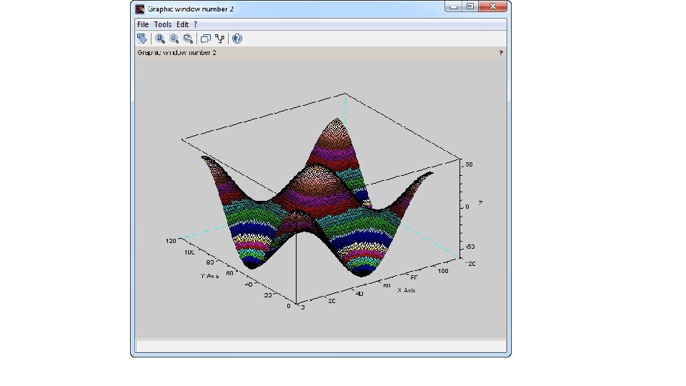
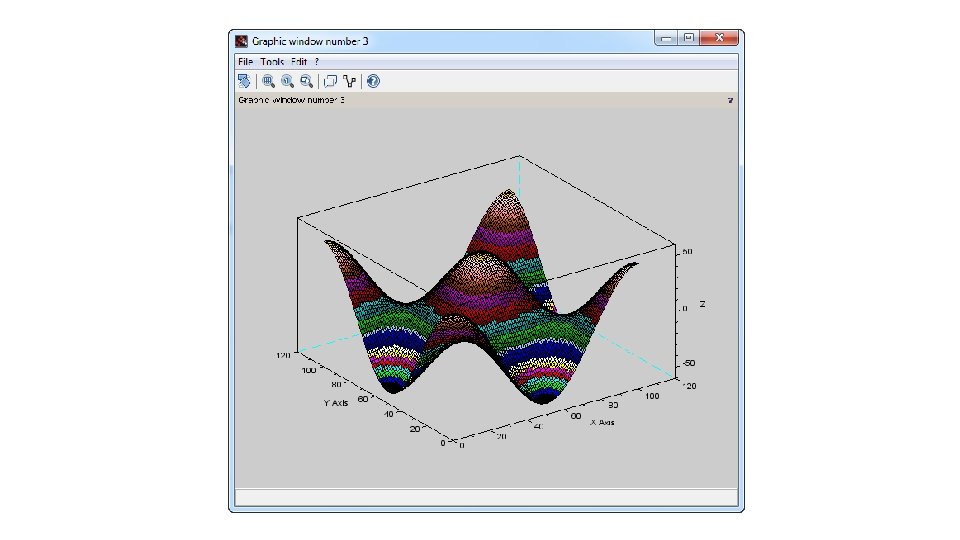
3. Step : Combine the codes. àa=0: 0. 01: 1; àb=sin(2*%pi*a); àc=cos(2*%pi*a); àd=b’*b; àe=e’*e; àfigure(1) àsurf(d) xlabel('X Axis') ylabel('Y Axis') figure(2) surf(e) xlabel('X Axis') ylabel('Y Axis')

Result

3 -D Multiple Image Subplot

16. 2 D Subplot 1. Step: First create the program for sine function. àa=0: 0. 01: 1; àb=sin(2*%pi*a); àc=b’*b; àsurf(c)
;")
2. Step : Write the program for cos wave. àa=0: 0. 01: 1; àb=cos(2*%pi*a); àc=b’*b; àsurf(c)
; àc=cos(2*%pi*a); àd=b’*b; àe=e’*e;")
3. Step : Combine the codes. àa=0: 0. 01: 1; àb=sin(2*%pi*a); àc=cos(2*%pi*a); àd=b’*b; àe=e’*e; àsubplot(1, 2, 1) àsurf(d) xlabel('x axis') ylabel('y axis') subplot(1, 2, 1) surf(e) xlabel('x axis') ylabel('Y Axis')

Result

4. 2 D Processing

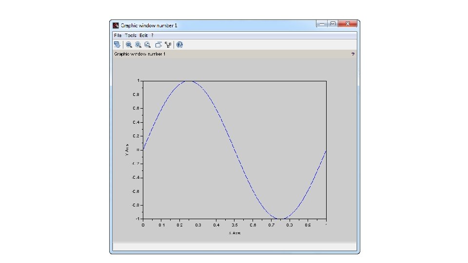
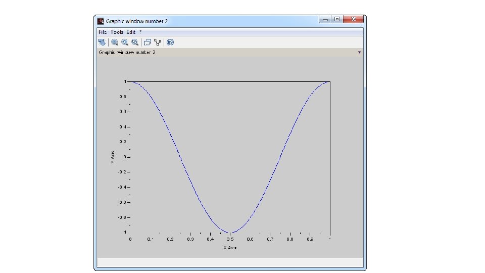
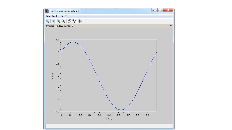
Create 3 D Sine and Cosine waves and add them to each other. a=0: 0. 01: 1; b=sin(2*%pi*a); c=cos(2*%pi*a); d=b+c; figure(1) plot(a, b) xlabel('X Axis') ylabel('Y Axis') figure(2) plot(a, c) xlabel('X Axis') ylabel('Y Axis') figure(3) plot(a, d) xlabel('X Axis') ylabel('Y Axis')

5. 3 D Processing

Create 3 D Sine and Cosine waves and add them to each other. a=0: 0. 01: 1; b=sin(2*%pi*a); c=cos(2*%pi*a); d=b’*b; e=e’*e; f=d+e; figure(1) surf(d) xlabel('X Axis') ylabel('Y Axis') figure(2) surf(e) xlabel('X Axis') ylabel('Y Axis') figure(3) surf(f) xlabel('X Axis') ylabel('Y Axis')

Thanks for your patience www. spectrumultra. com
- Slides: 79