Scientific Methods 1 Scientific evaluation experimental design statistical

Scientific Methods 1 ‘Scientific evaluation, experimental design & statistical methods’ COMP 80131 Lecture 4: Statistical Methods-Probability Barry & Goran www. cs. man. ac. uk/~barry/mydocs/my. COMP 80131 30 Nov 2012 COMP 80131 -SEEDSM 12 -4 1

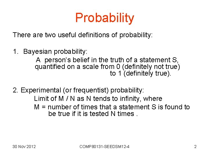
Probability There are two useful definitions of probability: 1. Bayesian probability: A person’s belief in the truth of a statement S, quantified on a scale from 0 (definitely not true) to 1 (definitely true). 2. Experimental (or frequentist) probability: Limit of M / N as N tends to infinity, where M = number of times that a statement S is found to be true if it is tested N times. 30 Nov 2012 COMP 80131 -SEEDSM 12 -4 2

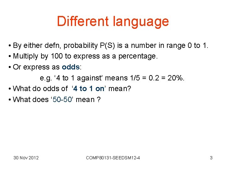
Different language • By either defn, probability P(S) is a number in range 0 to 1. • Multiply by 100 to express as a percentage. • Or express as odds: e. g. ‘ 4 to 1 against’ means 1/5 = 0. 2 = 20%. • What do odds of ‘ 4 to 1 on’ mean? • What does ‘ 50 -50’ mean ? 30 Nov 2012 COMP 80131 -SEEDSM 12 -4 3

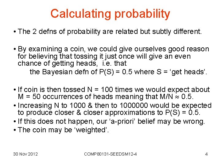
Calculating probability • The 2 defns of probability are related but subtly different. • By examining a coin, we could give ourselves good reason for believing that tossing it just once will give an even chance of getting heads, i. e. that the Bayesian defn of P(S) = 0. 5 where S = ‘get heads’. • If coin is then tossed N = 100 times we would expect about M = 50 occurrences of heads meaning that M/N 0. 5. • Increasing N to 1000 & then to 1000000 would be expected to produce closer & closer approximations to P(S) = 0. 5. • If this does not happen, our ‘a-priori’ belief may be wrong. • The coin may be ‘weighted’. 30 Nov 2012 COMP 80131 -SEEDSM 12 -4 4

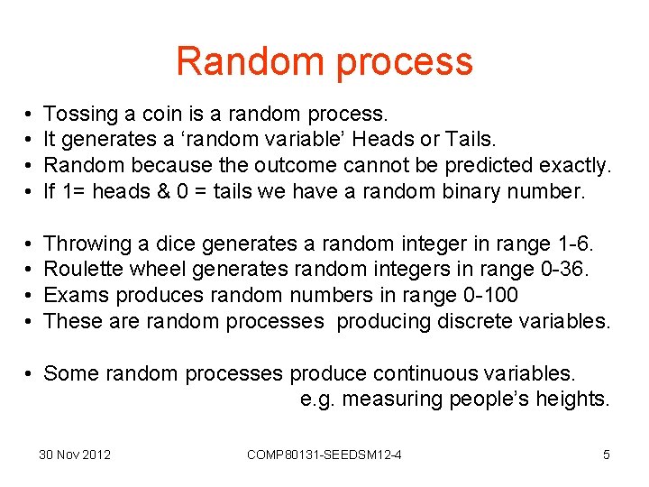
Random process • • Tossing a coin is a random process. It generates a ‘random variable’ Heads or Tails. Random because the outcome cannot be predicted exactly. If 1= heads & 0 = tails we have a random binary number. • • Throwing a dice generates a random integer in range 1 -6. Roulette wheel generates random integers in range 0 -36. Exams produces random numbers in range 0 -100 These are random processes producing discrete variables. • Some random processes produce continuous variables. e. g. measuring people’s heights. 30 Nov 2012 COMP 80131 -SEEDSM 12 -4 5

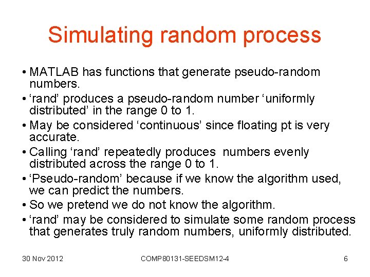
Simulating random process • MATLAB has functions that generate pseudo-random numbers. • ‘rand’ produces a pseudo-random number ‘uniformly distributed’ in the range 0 to 1. • May be considered ‘continuous’ since floating pt is very accurate. • Calling ‘rand’ repeatedly produces numbers evenly distributed across the range 0 to 1. • ‘Pseudo-random’ because if we know the algorithm used, we can predict the numbers. • So we pretend we do not know the algorithm. • ‘rand’ may be considered to simulate some random process that generates truly random numbers, uniformly distributed. 30 Nov 2012 COMP 80131 -SEEDSM 12 -4 6

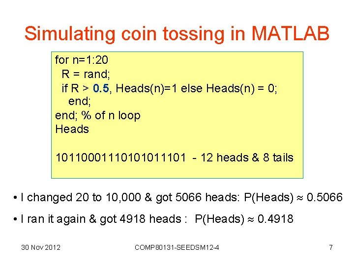
Simulating coin tossing in MATLAB for n=1: 20 R = rand; if R > 0. 5, Heads(n)=1 else Heads(n) = 0; end; % of n loop Heads 10110001110101011101 - 12 heads & 8 tails • I changed 20 to 10, 000 & got 5066 heads: P(Heads) 0. 5066 • I ran it again & got 4918 heads : P(Heads) 0. 4918 30 Nov 2012 COMP 80131 -SEEDSM 12 -4 7

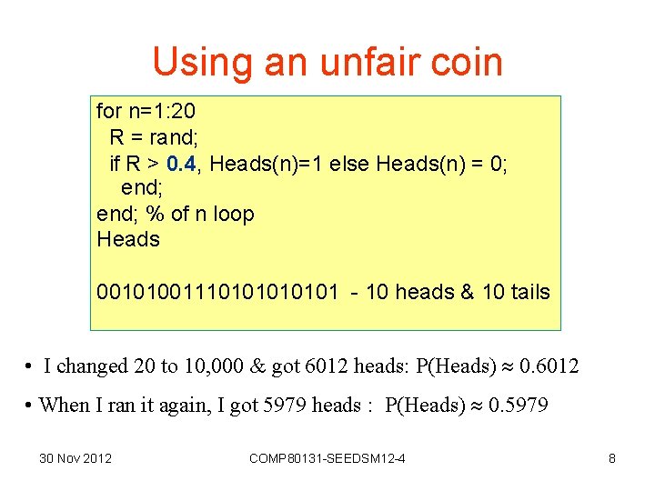
Using an unfair coin for n=1: 20 R = rand; if R > 0. 4, Heads(n)=1 else Heads(n) = 0; end; % of n loop Heads 0010100111010101 - 10 heads & 10 tails • I changed 20 to 10, 000 & got 6012 heads: P(Heads) 0. 6012 • When I ran it again, I got 5979 heads : P(Heads) 0. 5979 30 Nov 2012 COMP 80131 -SEEDSM 12 -4 8

Estimating probability experimentally • Cannot measure probability with 100% accuracy. • All measurements are estimates • They may be slightly or totally wrong. • According to experimental defn, we must perform an expt an infinite number of times to measure a probability. • This is clearly impossible. • In practice, we have to perform the experiment a finite number of times • (Cannot spend all our lives tossing coins) • Accept resulting measurement as estimate of true probability. 30 Nov 2012 COMP 80131 -SEEDSM 12 -4 9

Bayesian Definition • According to Bayesian defn of probability, a person’s belief in the truth of a statement may be affected by one or more assumption (hypotheses). • “I assume it is a fair coin” • Different people may have different beliefs. • Can only estimate probability using information we have available, • Can modify this estimate later if we get new information. 30 Nov 2012 COMP 80131 -SEEDSM 12 -4 10

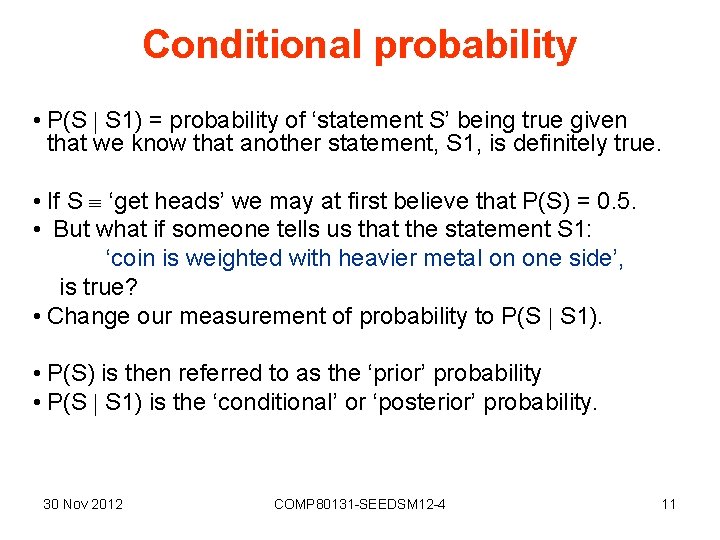
Conditional probability • P(S S 1) = probability of ‘statement S’ being true given that we know that another statement, S 1, is definitely true. • If S ‘get heads’ we may at first believe that P(S) = 0. 5. • But what if someone tells us that the statement S 1: ‘coin is weighted with heavier metal on one side’, is true? • Change our measurement of probability to P(S S 1). • P(S) is then referred to as the ‘prior’ probability • P(S S 1) is the ‘conditional’ or ‘posterior’ probability. 30 Nov 2012 COMP 80131 -SEEDSM 12 -4 11

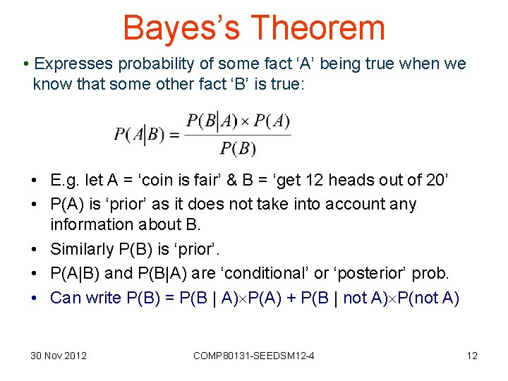
Bayes’s Theorem • Expresses probability of some fact ‘A’ being true when we know that some other fact ‘B’ is true: • E. g. let A = ‘coin is fair’ & B = ‘get 12 heads out of 20’ • P(A) is ‘prior’ as it does not take into account any information about B. • Similarly P(B) is ‘prior’. • P(A|B) and P(B|A) are ‘conditional’ or ‘posterior’ prob. • Can write P(B) = P(B | A) P(A) + P(B | not A) P(not A) 30 Nov 2012 COMP 80131 -SEEDSM 12 -4 12

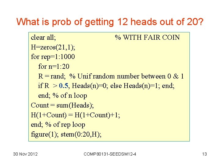
What is prob of getting 12 heads out of 20? clear all; % WITH FAIR COIN H=zeros(21, 1); for rep=1: 1000 for n=1: 20 R = rand; % Unif random number between 0 & 1 if R > 0. 5, Heads(n)=0; else Heads(n)=1; end; % of n loop Count = sum(Heads); H(1+Count) = H(1+Count)+1; end; % of rep loop figure(1); stem(0: 20, H); 30 Nov 2012 COMP 80131 -SEEDSM 12 -4 13

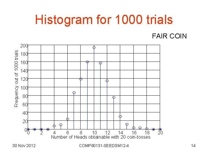
Histogram for 1000 trials FAIR COIN Frequency out of 1000 trials 200 180 160 140 120 100 80 60 40 20 0 0 30 Nov 2012 2 4 6 8 10 12 14 16 18 Number of Heads obtainable with 20 coin-tosses COMP 80131 -SEEDSM 12 -4 20 14

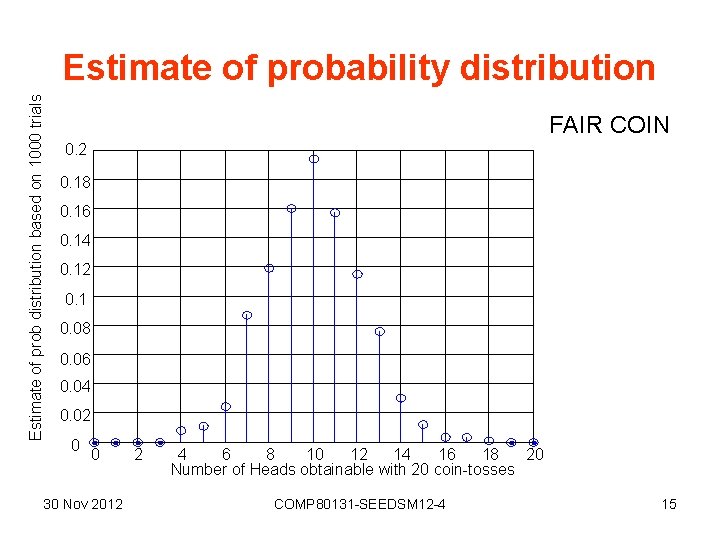
Estimate of prob distribution based on 1000 trials Estimate of probability distribution FAIR COIN 0. 2 0. 18 0. 16 0. 14 0. 12 0. 1 0. 08 0. 06 0. 04 0. 02 0 0 30 Nov 2012 2 4 6 8 10 12 14 16 18 20 Number of Heads obtainable with 20 coin-tosses COMP 80131 -SEEDSM 12 -4 15

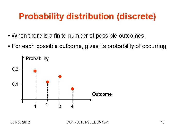
Probability distribution (discrete) • When there is a finite number of possible outcomes, • For each possible outcome, gives its probability of occurring. Probability 0. 2 0. 1 Outcome 1 30 Nov 2012 2 3 4 COMP 80131 -SEEDSM 12 -4 16

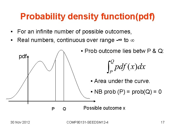
Probability density function(pdf) • For an infinite number of possible outcomes, • Real numbers, continuous over range -∞ to • Prob outcome lies betw P & Q: pdf • Area under the curve. • NB prob (P) = prob(Q) = 0 P 30 Nov 2012 Q Possible outcome x COMP 80131 -SEEDSM 12 -4 17

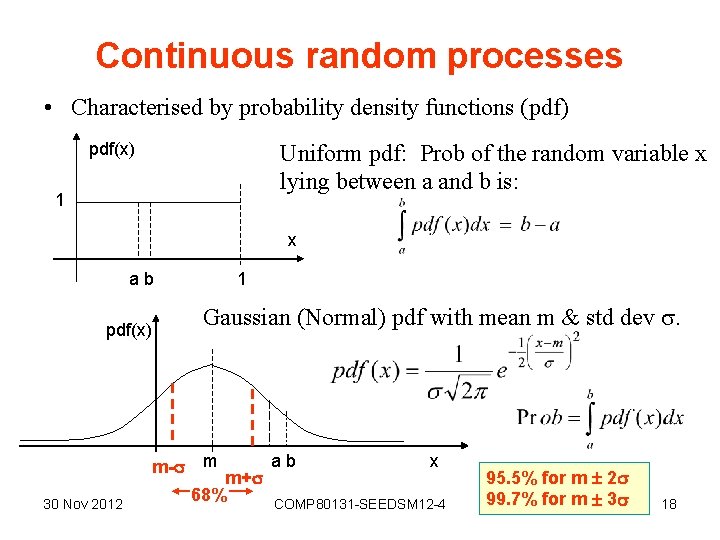
Continuous random processes • Characterised by probability density functions (pdf) pdf(x) Uniform pdf: Prob of the random variable x lying between a and b is: 1 x ab pdf(x) m- 30 Nov 2012 1 Gaussian (Normal) pdf with mean m & std dev . m m+ 68% ab x COMP 80131 -SEEDSM 12 -4 95. 5% for m 2 99. 7% for m 3 18

Continuous distributions • More about these later. • Back to discrete now. 30 Nov 2012 COMP 80131 -SEEDSM 12 -4 19

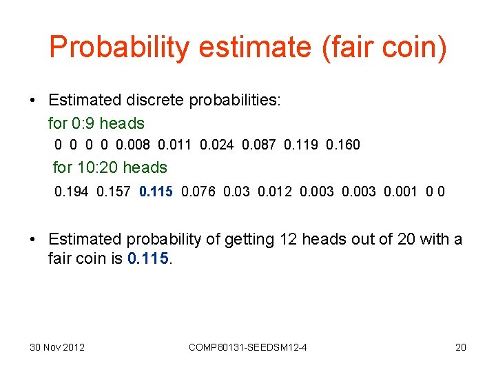
Probability estimate (fair coin) • Estimated discrete probabilities: for 0: 9 heads 0 0 0. 008 0. 011 0. 024 0. 087 0. 119 0. 160 for 10: 20 heads 0. 194 0. 157 0. 115 0. 076 0. 03 0. 012 0. 003 0. 001 0 0 • Estimated probability of getting 12 heads out of 20 with a fair coin is 0. 115. 30 Nov 2012 COMP 80131 -SEEDSM 12 -4 20

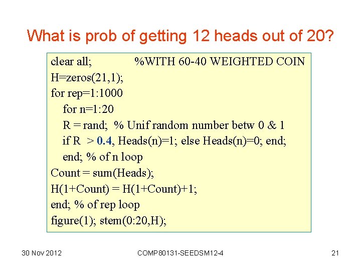
What is prob of getting 12 heads out of 20? clear all; %WITH 60 -40 WEIGHTED COIN H=zeros(21, 1); for rep=1: 1000 for n=1: 20 R = rand; % Unif random number betw 0 & 1 if R > 0. 4, Heads(n)=1; else Heads(n)=0; end; % of n loop Count = sum(Heads); H(1+Count) = H(1+Count)+1; end; % of rep loop figure(1); stem(0: 20, H); 30 Nov 2012 COMP 80131 -SEEDSM 12 -4 21

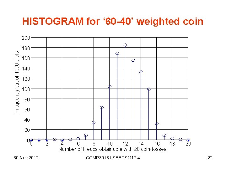
HISTOGRAM for ‘ 60 -40’ weighted coin 200 Frequency out of 1000 trials 180 160 140 120 100 80 60 40 20 0 0 30 Nov 2012 2 4 6 8 10 12 14 16 18 Number of Heads obtainable with 20 coin-tosses COMP 80131 -SEEDSM 12 -4 20 22

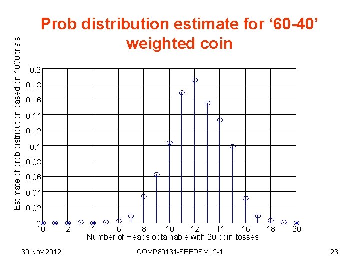
Estimate of prob distribution based on 1000 trials Prob distribution estimate for ‘ 60 -40’ weighted coin 0. 2 0. 18 0. 16 0. 14 0. 12 0. 1 0. 08 0. 06 0. 04 0. 02 0 0 30 Nov 2012 2 4 6 8 10 12 14 16 18 Number of Heads obtainable with 20 coin-tosses COMP 80131 -SEEDSM 12 -4 20 23

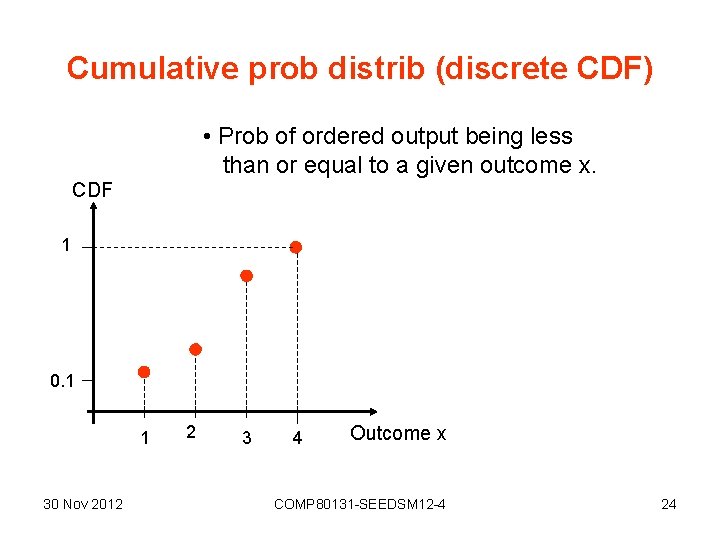
Cumulative prob distrib (discrete CDF) • Prob of ordered output being less than or equal to a given outcome x. CDF 1 0. 1 1 30 Nov 2012 2 3 4 Outcome x COMP 80131 -SEEDSM 12 -4 24

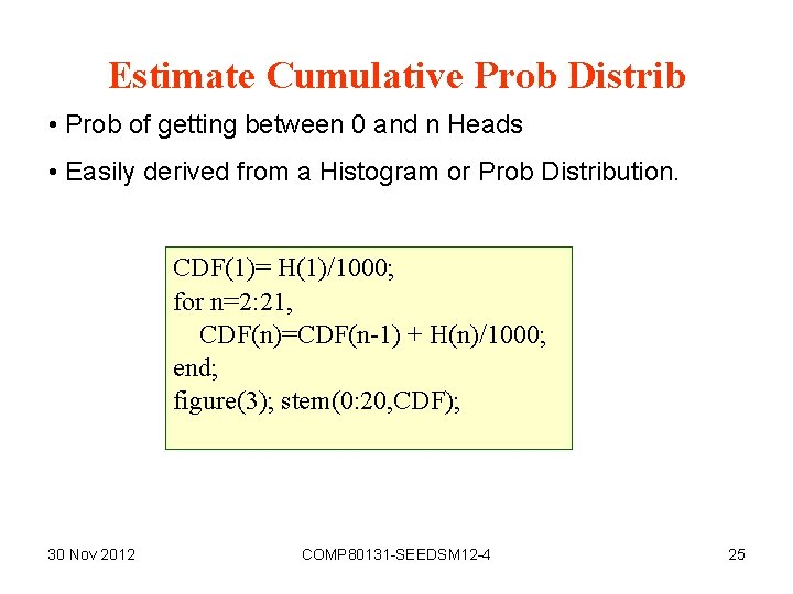
Estimate Cumulative Prob Distrib • Prob of getting between 0 and n Heads • Easily derived from a Histogram or Prob Distribution. CDF(1)= H(1)/1000; for n=2: 21, CDF(n)=CDF(n-1) + H(n)/1000; end; figure(3); stem(0: 20, CDF); 30 Nov 2012 COMP 80131 -SEEDSM 12 -4 25

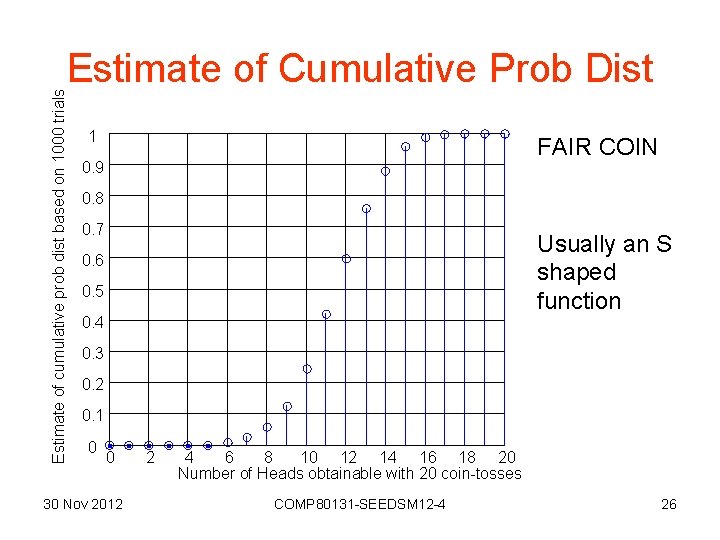
Estimate of cumulative prob dist based on 1000 trials Estimate of Cumulative Prob Dist 1 FAIR COIN 0. 9 0. 8 0. 7 Usually an S shaped function 0. 6 0. 5 0. 4 0. 3 0. 2 0. 1 0 0 30 Nov 2012 2 4 6 8 10 12 14 16 18 20 Number of Heads obtainable with 20 coin-tosses COMP 80131 -SEEDSM 12 -4 26

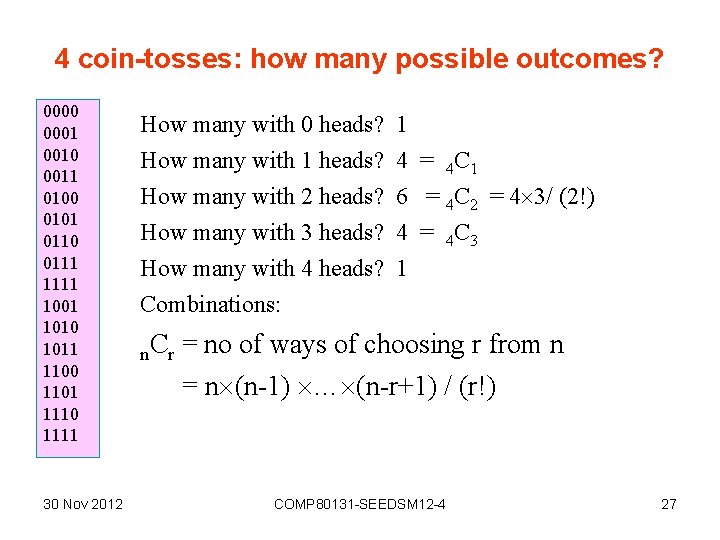
4 coin-tosses: how many possible outcomes? 0000 0001 0010 0011 0100 0101 0110 0111 1001 1010 1011 1100 1101 1110 1111 30 Nov 2012 How many with 0 heads? 1 How many with 1 heads? How many with 2 heads? How many with 3 heads? How many with 4 heads? Combinations: n. Cr 4 = 4 C 1 6 = 4 C 2 = 4 3/ (2!) 4 = 4 C 3 1 = no of ways of choosing r from n = n (n-1) … (n-r+1) / (r!) COMP 80131 -SEEDSM 12 -4 27

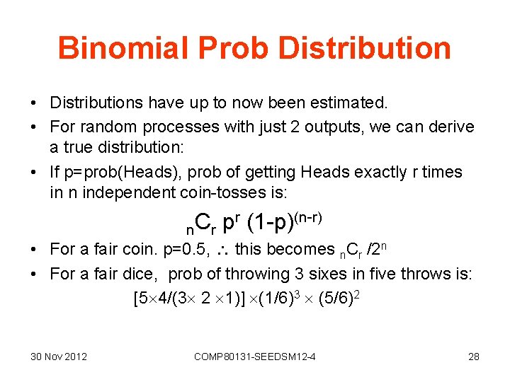
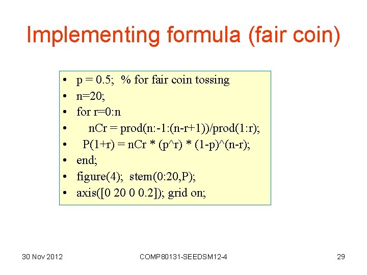
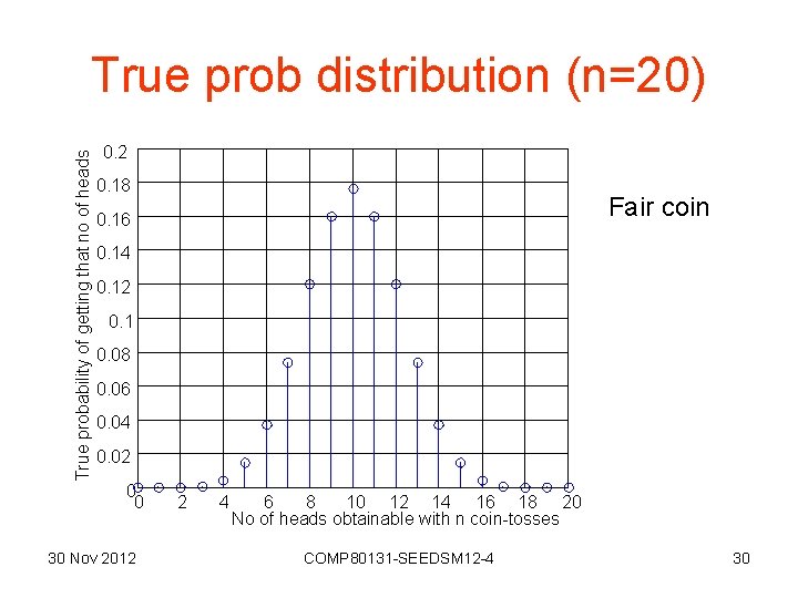
Binomial Prob Distribution • Distributions have up to now been estimated. • For random processes with just 2 outputs, we can derive a true distribution: • If p=prob(Heads), prob of getting Heads exactly r times in n independent coin-tosses is: r (1 -p)(n-r) C p n r • For a fair coin. p=0. 5, this becomes n. Cr /2 n • For a fair dice, prob of throwing 3 sixes in five throws is: [5 4/(3 2 1)] (1/6)3 (5/6)2 30 Nov 2012 COMP 80131 -SEEDSM 12 -4 28

Implementing formula (fair coin) • • 30 Nov 2012 p = 0. 5; % for fair coin tossing n=20; for r=0: n n. Cr = prod(n: -1: (n-r+1))/prod(1: r); P(1+r) = n. Cr * (p^r) * (1 -p)^(n-r); end; figure(4); stem(0: 20, P); axis([0 20 0 0. 2]); grid on; COMP 80131 -SEEDSM 12 -4 29

True probability of getting that no of heads True prob distribution (n=20) 0. 2 0. 18 Fair coin 0. 16 0. 14 0. 12 0. 1 0. 08 0. 06 0. 04 0. 02 0 0 30 Nov 2012 2 4 6 8 10 12 14 16 18 20 No of heads obtainable with n coin-tosses COMP 80131 -SEEDSM 12 -4 30

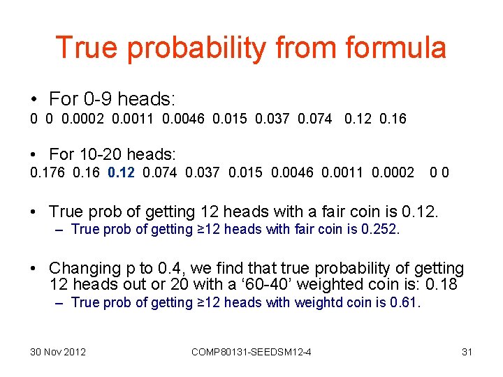
True probability from formula • For 0 -9 heads: 0 0 0. 0002 0. 0011 0. 0046 0. 015 0. 037 0. 074 0. 12 0. 16 • For 10 -20 heads: 0. 176 0. 12 0. 074 0. 037 0. 015 0. 0046 0. 0011 0. 0002 00 • True prob of getting 12 heads with a fair coin is 0. 12. – True prob of getting ≥ 12 heads with fair coin is 0. 252. • Changing p to 0. 4, we find that true probability of getting 12 heads out or 20 with a ‘ 60 -40’ weighted coin is: 0. 18 – True prob of getting ≥ 12 heads with weightd coin is 0. 61. 30 Nov 2012 COMP 80131 -SEEDSM 12 -4 31

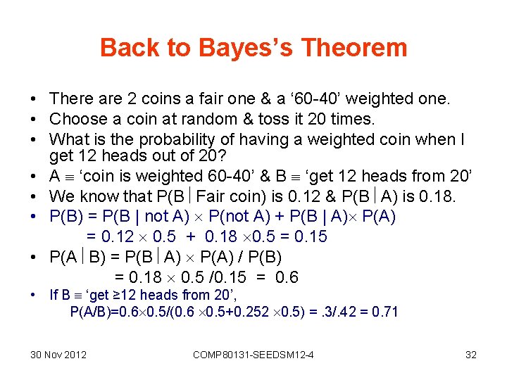
Back to Bayes’s Theorem • There are 2 coins a fair one & a ‘ 60 -40’ weighted one. • Choose a coin at random & toss it 20 times. • What is the probability of having a weighted coin when I get 12 heads out of 20? • A ‘coin is weighted 60 -40’ & B ‘get 12 heads from 20’ • We know that P(B Fair coin) is 0. 12 & P(B A) is 0. 18. • P(B) = P(B | not A) P(not A) + P(B | A) P(A) = 0. 12 0. 5 + 0. 18 0. 5 = 0. 15 • P(A B) = P(B A) P(A) / P(B) = 0. 18 0. 5 /0. 15 = 0. 6 • If B ‘get ≥ 12 heads from 20’, P(A/B)=0. 6 0. 5/(0. 6 0. 5+0. 252 0. 5) =. 3/. 42 = 0. 71 30 Nov 2012 COMP 80131 -SEEDSM 12 -4 32

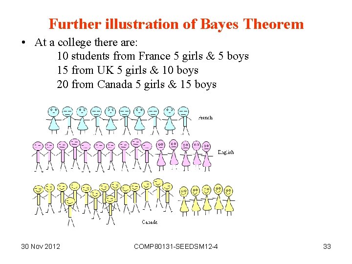
Further illustration of Bayes Theorem • At a college there are: 10 students from France 5 girls & 5 boys 15 from UK 5 girls & 10 boys 20 from Canada 5 girls & 15 boys 30 Nov 2012 COMP 80131 -SEEDSM 12 -4 33

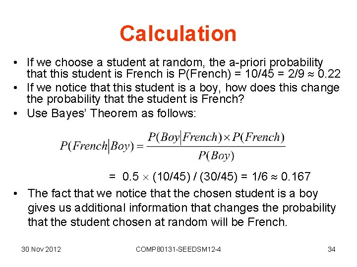
Calculation • If we choose a student at random, the a-priori probability that this student is French is P(French) = 10/45 = 2/9 0. 22 • If we notice that this student is a boy, how does this change the probability that the student is French? • Use Bayes’ Theorem as follows: = 0. 5 (10/45) / (30/45) = 1/6 0. 167 • The fact that we notice that the chosen student is a boy gives us additional information that changes the probability that the student chosen at random will be French. 30 Nov 2012 COMP 80131 -SEEDSM 12 -4 34

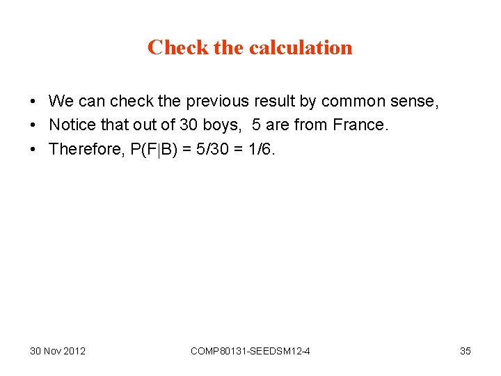
Check the calculation • We can check the previous result by common sense, • Notice that out of 30 boys, 5 are from France. • Therefore, P(F B) = 5/30 = 1/6. 30 Nov 2012 COMP 80131 -SEEDSM 12 -4 35

Usefulness of Bayes Theorem • It allows us to take additional information into account when calculating probabilities. • Without the additional information, we have a ‘prior’ probability • With it we have a ‘conditional’ or ‘posterior’ probability. 30 Nov 2012 COMP 80131 -SEEDSM 12 -4 36

Bayes Theorem in medicine • A patent goes to a doctor with a bad cough & a fever. The doctor needs to decide whether he has ‘swine flu’. • Let statement S = ‘has bad cough and fever’ and statement F = ‘has swine flu’. • The doctor consults his medical books and finds that about 40% of patients with swine-flu have these same symptoms. • Assuming that, currently, about 1% of the population is suffering from swine-flu and that currently about 5% have bad cough and fever (due to many possible causes including swine-flu), we can apply Bayes theorem to estimate the probability of this particular patient having swine-flu. 30 Nov 2012 COMP 80131 -SEEDSM 12 -4 37

Another problem to solve • A doctor in another country knows form his text-books that for 40% of patients with swine-flu, • The statement S, ‘has bad cough and fever’ is true. • He sees many patients and comes to believe that the probability that a patient with ‘bad cough and fever’ actually has swine-flu is about 0. 1 or 10%. • If there were reason to believe that, currently, about 1% of the population have a bad cough and fever, what percentage of the population is likely to be suffering from swine-flu? 30 Nov 2012 COMP 80131 -SEEDSM 12 -4 38

Concept of a ‘null-hypothesis’ • A null-hypothesis is an assumption that is made and then tested by a set of experiments designed to reveal that it is likely to be false, if it is false. • Testing is done by considering how probable the results are, assuming the null hypothesis is true. • If the results appear very improbable the researcher may conclude that the null-hypothesis is likely to be false. • This is usually the outcome the researcher hopes for when he or she is trying to prove that a new technique is likely to have some value. 30 Nov 2012 COMP 80131 -SEEDSM 12 -4 39

An example • Assume we wish to find out if a proposed technique designed to benefit users of a system is likely to have any value. • Divide the users into two groups and offer the proposed technique to one group and something different to the other group. • The null-hypothesis would be that the proposed technique offers no measurable advantage over the other techniques. 30 Nov 2012 COMP 80131 -SEEDSM 12 -4 40

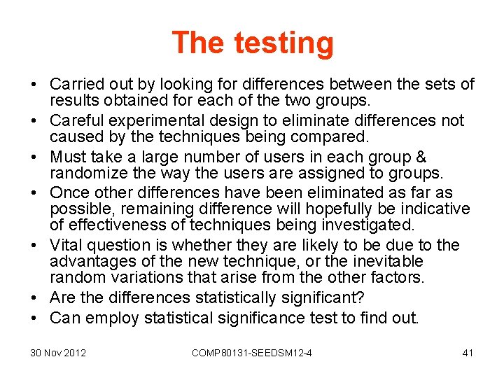
The testing • Carried out by looking for differences between the sets of results obtained for each of the two groups. • Careful experimental design to eliminate differences not caused by the techniques being compared. • Must take a large number of users in each group & randomize the way the users are assigned to groups. • Once other differences have been eliminated as far as possible, remaining difference will hopefully be indicative of effectiveness of techniques being investigated. • Vital question is whether they are likely to be due to the advantages of the new technique, or the inevitable random variations that arise from the other factors. • Are the differences statistically significant? • Can employ statistical significance test to find out. 30 Nov 2012 COMP 80131 -SEEDSM 12 -4 41

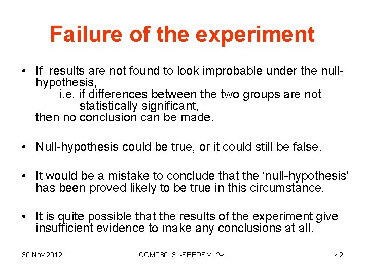
Failure of the experiment • If results are not found to look improbable under the nullhypothesis, i. e. if differences between the two groups are not statistically significant, then no conclusion can be made. • Null-hypothesis could be true, or it could still be false. • It would be a mistake to conclude that the ‘null-hypothesis’ has been proved likely to be true in this circumstance. • It is quite possible that the results of the experiment give insufficient evidence to make any conclusions at all. 30 Nov 2012 COMP 80131 -SEEDSM 12 -4 42

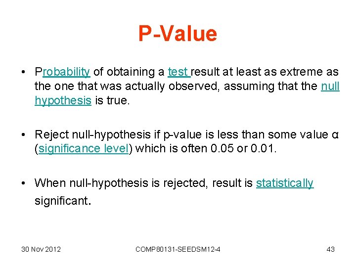
P-Value • Probability of obtaining a test result at least as extreme as the one that was actually observed, assuming that the null hypothesis is true. • Reject null-hypothesis if p-value is less than some value α (significance level) which is often 0. 05 or 0. 01. • When null-hypothesis is rejected, result is statistically significant. 30 Nov 2012 COMP 80131 -SEEDSM 12 -4 43

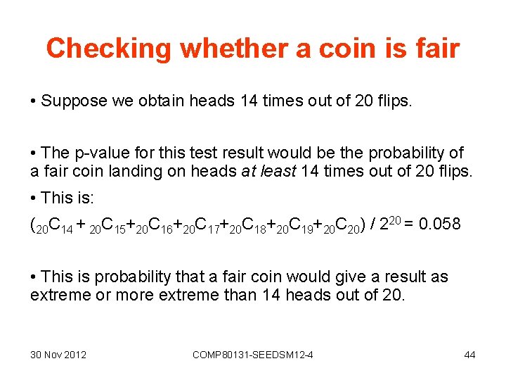
Checking whether a coin is fair • Suppose we obtain heads 14 times out of 20 flips. • The p-value for this test result would be the probability of a fair coin landing on heads at least 14 times out of 20 flips. • This is: (20 C 14 + 20 C 15+20 C 16+20 C 17+20 C 18+20 C 19+20 C 20) / 220 = 0. 058 • This is probability that a fair coin would give a result as extreme or more extreme than 14 heads out of 20. 30 Nov 2012 COMP 80131 -SEEDSM 12 -4 44

Significance test • Reject null-hypothesis if p-value α. • If α= 0. 05, rejection of null-hypothesis is at the 5% (significance) level. • Probability of wrongly rejecting null-hypothesis (Type 1 error) will be equal to α. • This is considered ‘sufficiently low’. • In this ‘coin testing’ case, p-value > 0. 05, • Therefore observation is consistent with null-hypothesis and we cannot reject it. • Cannot conclude that coin is likely to be unfair. • But we have NOT proved that coin is likely to be fair. • 14 heads out of 20 flips can be ascribed to chance alone. • It falls within the range of what could happen 95% of the time with a fair coin. 30 Nov 2012 COMP 80131 -SEEDSM 12 -4 45