Scientific Computation Using Excel 1 Introduction Scientific computing

Scientific Computation Using Excel 1. Introduction Scientific computing is very important for solving real world application problems. Population predictions, financial decisions, curve fitting, fixed point iterations, numerical solutions to differential equations require scientific computation. Excel is a very useful and easy to use software to perform these computations.

Difference Equation 2. Difference Equation A difference equation is an equation relating successive terms of a sequence. The solution to the difference equation is the sequence (a function of n ) that satisfies the difference equation. While it can always be expressed in terms of the specific numbers in the sequence, whenever possible, it is desirable to express the solution as a formula in closed form in terms of the general term.

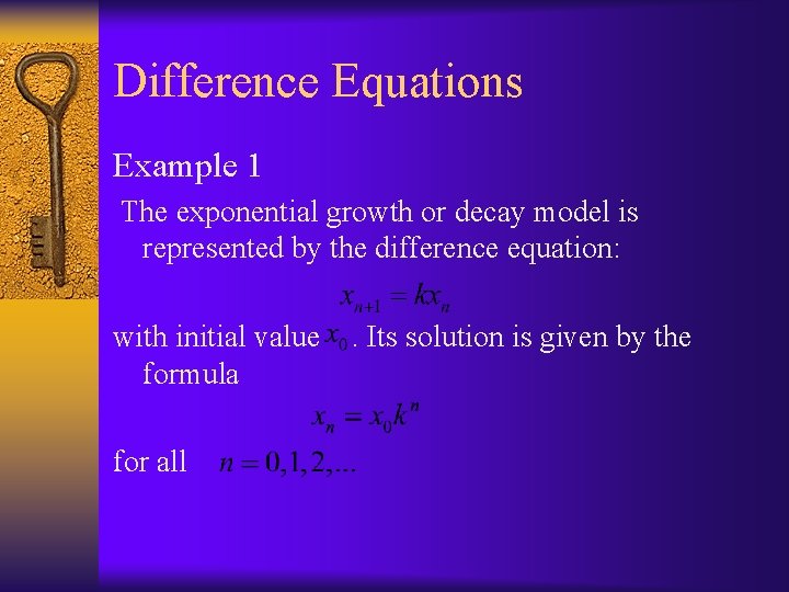
Difference Equations Example 1 The exponential growth or decay model is represented by the difference equation: with initial value . Its solution is given by the formula for all

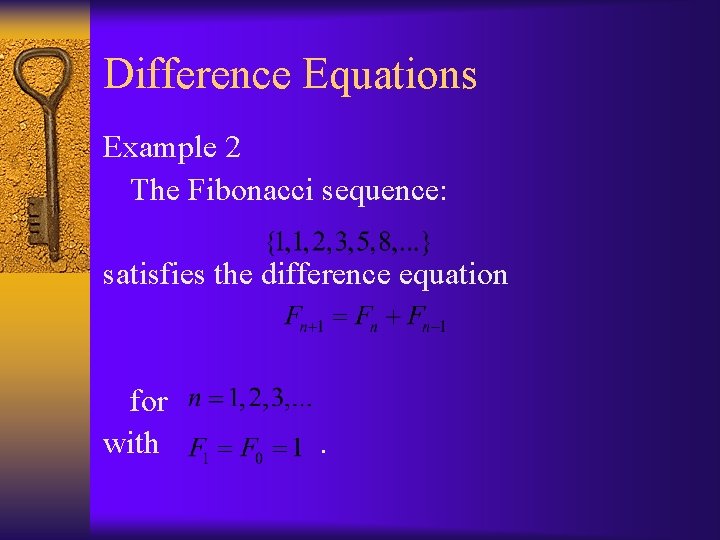
Difference Equations Example 2 The Fibonacci sequence: satisfies the difference equation for with .

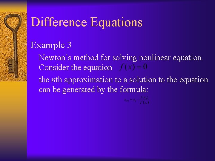
Difference Equations Example 3 Newton’s method for solving nonlinear equation. Consider the equation the nth approximation to a solution to the equation can be generated by the formula:

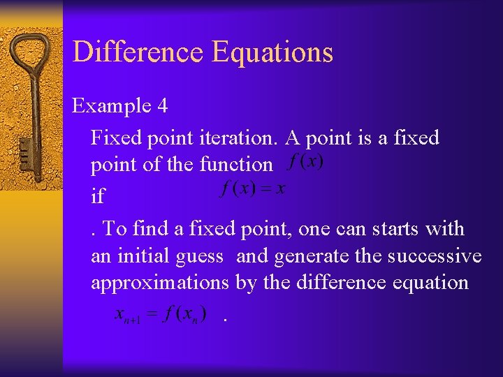
Difference Equations Example 4 Fixed point iteration. A point is a fixed point of the function if . To find a fixed point, one can starts with an initial guess and generate the successive approximations by the difference equation .

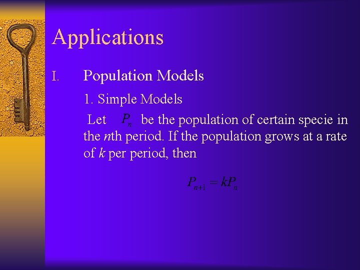
Applications I. Population Models 1. Simple Models Let be the population of certain specie in the nth period. If the population grows at a rate of k period, then

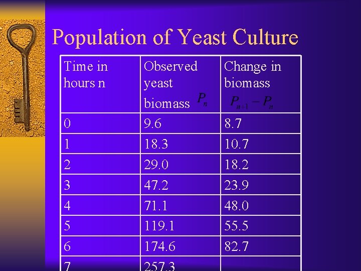
Population of Yeast Culture Time in hours n 0 1 2 3 4 5 6 Observed yeast biomass 9. 6 18. 3 29. 0 47. 2 71. 1 119. 1 174. 6 Change in biomass 8. 7 10. 7 18. 2 23. 9 48. 0 55. 5 82. 7

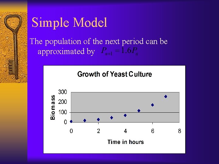
Simple Model The population of the next period can be approximated by

Simple Model

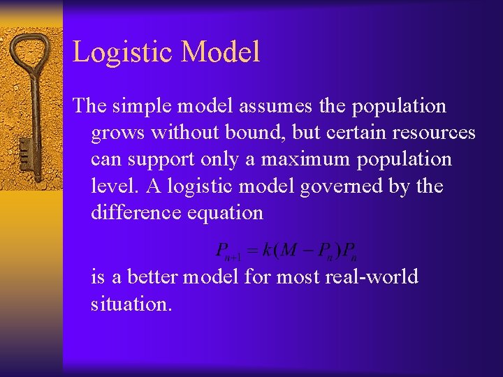
Logistic Model The simple model assumes the population grows without bound, but certain resources can support only a maximum population level. A logistic model governed by the difference equation is a better model for most real-world situation.

The Graph of a Yeast Culture

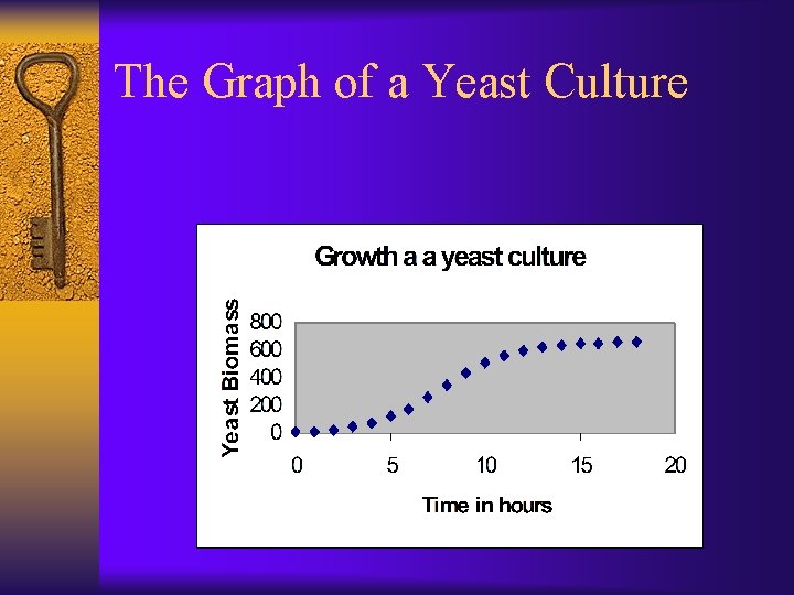
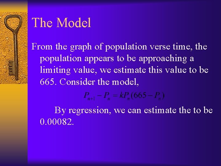
The Model From the graph of population verse time, the population appears to be approaching a limiting value, we estimate this value to be 665. Consider the model, By regression, we can estimate the to be 0. 00082.

Financing a Car or a Home You want to buy a car or a home by financing. Every one will tell you this is a good time to do it. A mortgage company will loan you a certain amount of money with a fixed annual interest rate , now you will repay this debt with a series of equal monthly payments over a fixed number of months. There are several questions that you, as a consumer, should be able to answer:

Financing a Car or a Home ¨ a. Given the loan amount, the term, the interest rate, how much will be the monthly payment? ¨ b. Given the term of the loan, the interest rate. If you know how much you can pay for each month, what will be the maximum amount of loan that you can afford to? ¨ c. For each month, how much of your monthly payment is going into the principal? How much is paying for the interests?

A Car Rental Model Consider a car rental company with distributorships in Orlando and Tampa. The company specializes in catering to travel agents who wants to arrange tourist activities in both Orlando and Tampa. Consequently, a traveler will rent a car in one city and drop the car off in the second city. Travelers may begin their itinerary in either city. The company is trying to determine how much to charge for this drop-off convenience.

A Car Rental Model Because cars are dropped off in both cities, will a sufficient number of cars end up in each city to satisfy the demand for cars in that city? If not, how many cars must be the company transport from Orlando to Tampa or from Tampa to Orlando? The answers to these questions will help the company figure out the expected costs

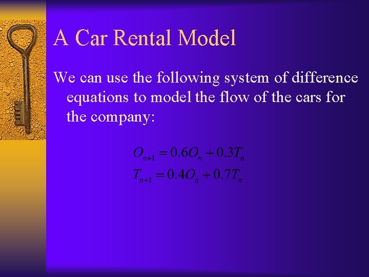
A Car Rental Model The historical records suggest that 60% of the cars rented in Orlando are returned to Orlando, whereas the other 40% of the cars end up in Tampa. Of the cars rented in Tampa, 70% are returned to Tampa, whereas the 30% end up in Orlando. Define the number of cars in Orlando at the end of day the number of cars in Tampa at the end of day .

A Car Rental Model We can use the following system of difference equations to model the flow of the cars for the company:

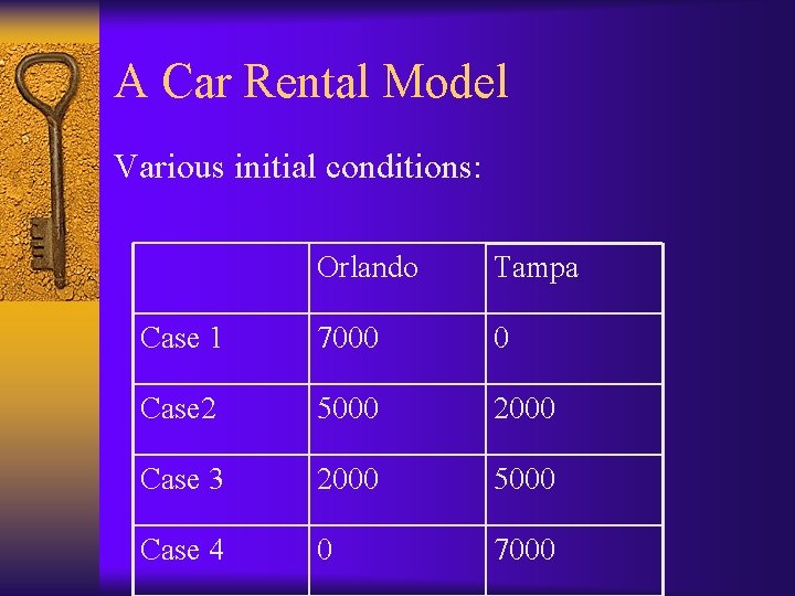
A Car Rental Model Various initial conditions: Orlando Tampa Case 1 7000 0 Case 2 5000 2000 Case 3 2000 5000 Case 4 0 7000

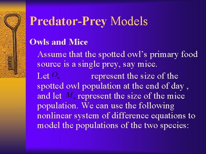
Predator-Prey Models Owls and Mice Assume that the spotted owl’s primary food source is a single prey, say mice. Let represent the size of the spotted owl population at the end of day , and let represent the size of the mice population. We can use the following nonlinear system of difference equations to model the populations of the two species:

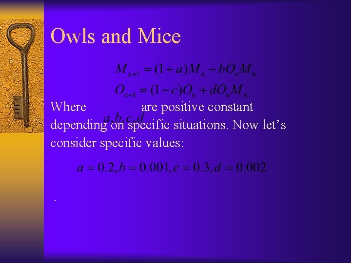
Owls and Mice Where are positive constant depending on specific situations. Now let’s consider specific values: .

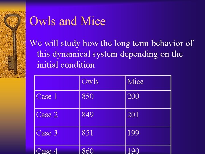
Owls and Mice We will study how the long term behavior of this dynamical system depending on the initial condition Owls Mice Case 1 850 200 Case 2 849 201 Case 3 851 199 Case 4 860 190

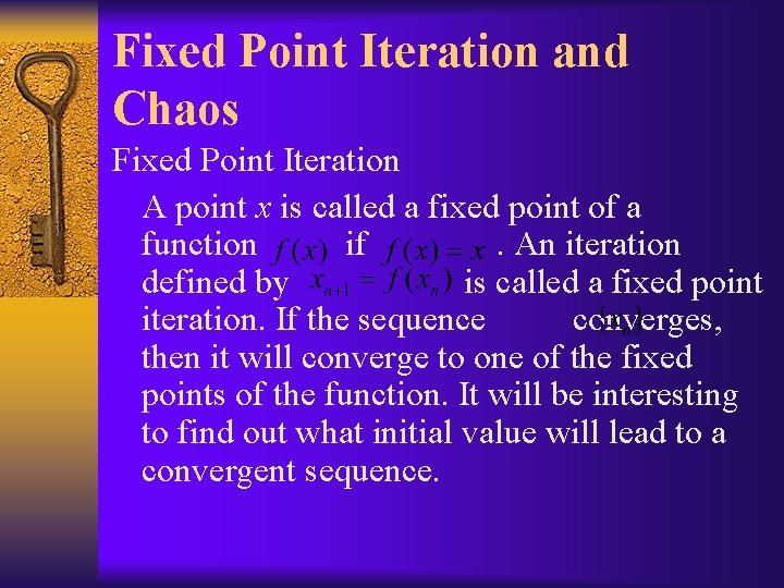
Fixed Point Iteration and Chaos Fixed Point Iteration A point x is called a fixed point of a function if . An iteration defined by is called a fixed point iteration. If the sequence converges, then it will converge to one of the fixed points of the function. It will be interesting to find out what initial value will lead to a convergent sequence.

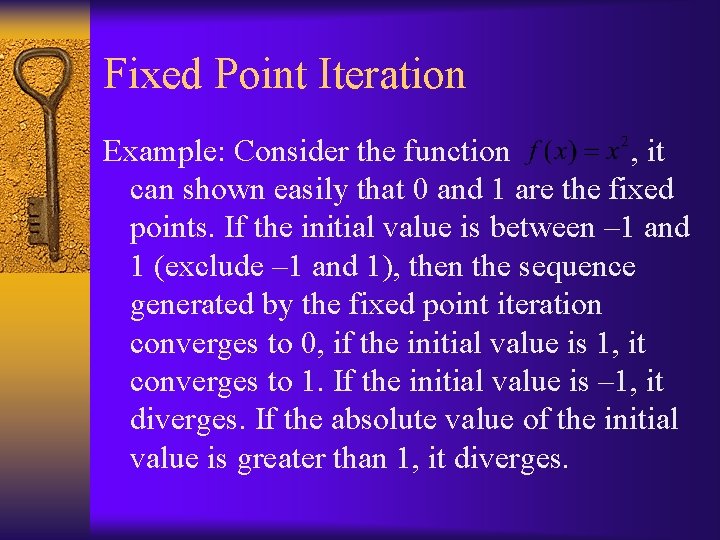
Fixed Point Iteration Example: Consider the function , it can shown easily that 0 and 1 are the fixed points. If the initial value is between – 1 and 1 (exclude – 1 and 1), then the sequence generated by the fixed point iteration converges to 0, if the initial value is 1, it converges to 1. If the initial value is – 1, it diverges. If the absolute value of the initial value is greater than 1, it diverges.

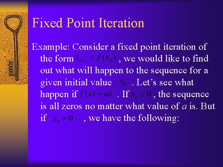
Fixed Point Iteration Example: Consider a fixed point iteration of the form , we would like to find out what will happen to the sequence for a given initial value . Let’s see what happen if . If , the sequence is all zeros no matter what value of a is. But if , we have the following:

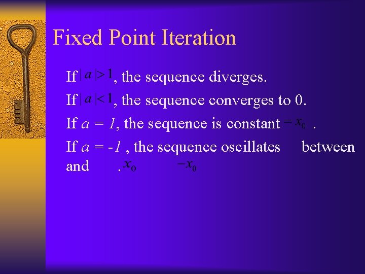
Fixed Point Iteration If , the sequence diverges. If , the sequence converges to 0. If a = 1, the sequence is constant . If a = -1 , the sequence oscillates between and .

Chaos Example: Now let us explore what will happen if First, if the initial value is 0, then all successive iterates are 0. Second, if any iterate is either 0 or 1, then all successive iterates will remain 0. Third, if any iterate is negative, then the succeeding value will also be negative;

Chaos further, will be more negative than because of the term . Consequently, the successive term will diverge toward . Fourth, if any iterate is larger than 1, then the succeeding value will be negative and the sequence will thereafter diverge to . As a result, we see that the only meaningful cases involve starting with values between 0 and 1 and remaining there for all values of thereafter.

Chaos Now let us see what effect the value a of has on the process. You can study this using Excel. We will explore what will happen to the sequence if a between 0 and 1, between 1 and 3, between 3 and 4, greater than 4.