SCHISM Crossscale Modeling System Opensource community supported system

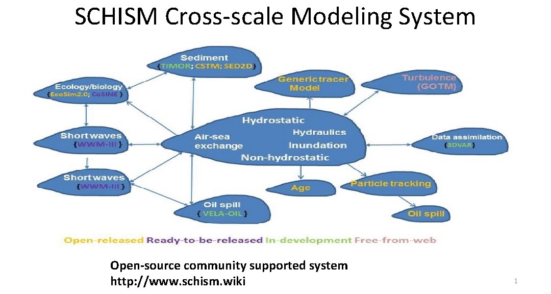
SCHISM Cross-scale Modeling System Open-source community supported system http: //www. schism. wiki 1

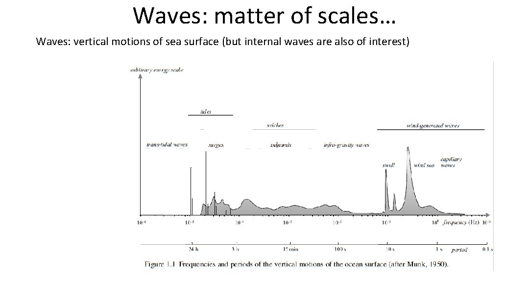
Waves: matter of scales… Waves: vertical motions of sea surface (but internal waves are also of interest)

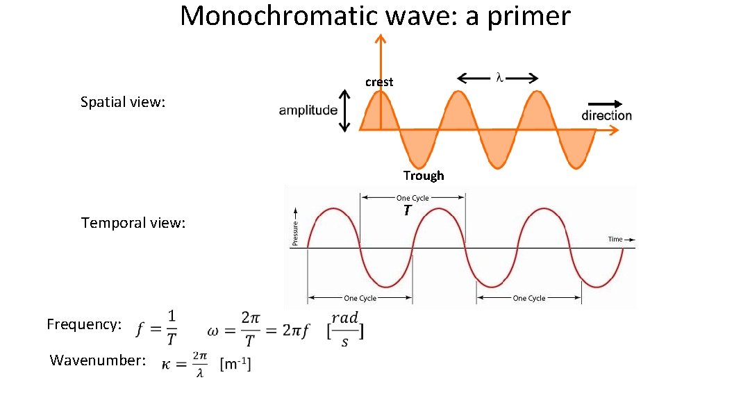
Monochromatic wave: a primer crest Spatial view: Trough T Temporal view: Frequency: Wavenumber:

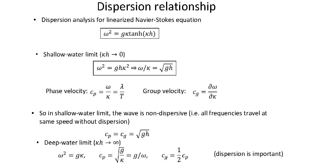
Dispersion relationship • Dispersion analysis for linearized Navier-Stokes equation Phase velocity: Group velocity: • So in shallow-water limit, the wave is non-dispersive (i. e. all frequencies travel at same speed without dispersion) (dispersion is important)

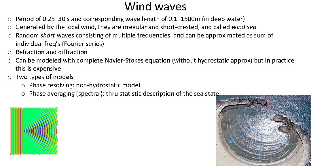
Wind waves o Period of 0. 25– 30 s and corresponding wave length of 0. 1– 1500 m (in deep water) o Generated by the local wind, they are irregular and short-crested, and called wind sea o Random short waves consisting of multiple frequencies, and can be approximated as sum of individual freq’s (Fourier series) o Refraction and diffraction o Can be modeled with complete Navier-Stokes equation (without hydrostatic approx) but in practice this is expensive o Two types of models o Phase resolving: non-hydrostatic model o Phase averaging (spectral): thru statistic description of the sea state

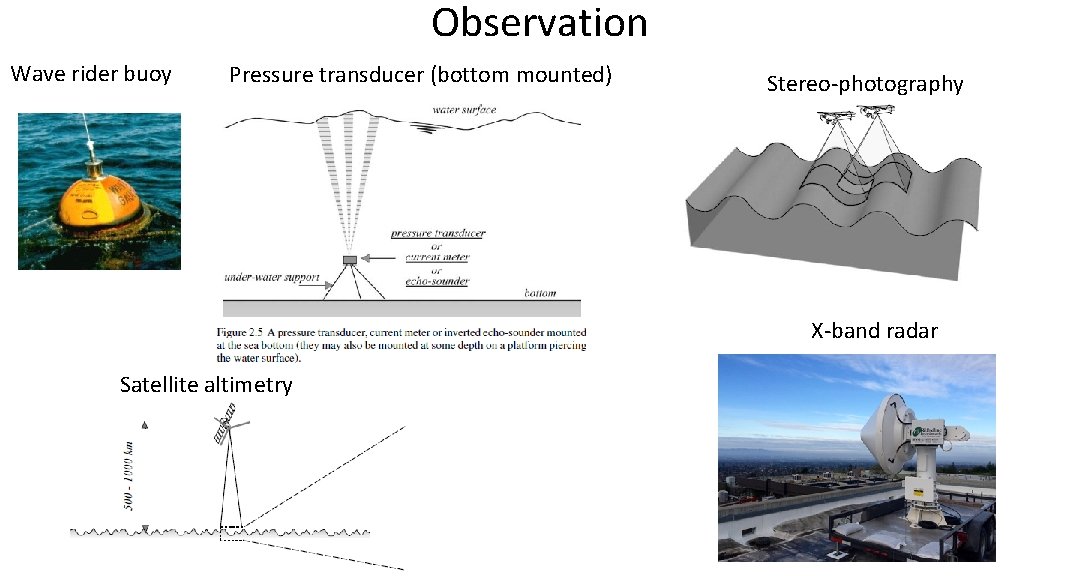
Observation Wave rider buoy Pressure transducer (bottom mounted) Stereo-photography X-band radar Satellite altimetry

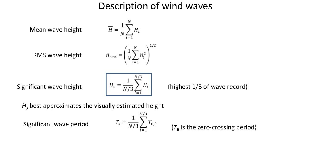
Description of wind waves Mean wave height RMS wave height Significant wave height i (highest 1/3 of wave record) Hs best approximates the visually estimated height Significant wave period (T 0 is the zero-crossing period)

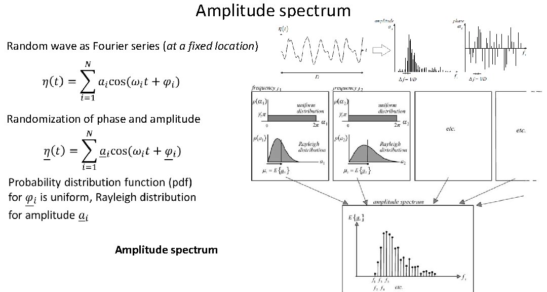
Amplitude spectrum Random wave as Fourier series (at a fixed location) Randomization of phase and amplitude Amplitude spectrum

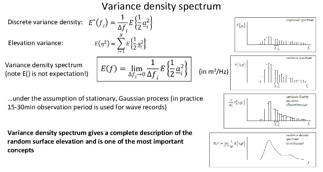
Variance density spectrum Discrete variance density: Elevation variance: Variance density spectrum (note E() is not expectation!) (in m 2/Hz) …under the assumption of stationary, Gaussian process (in practice 15 -30 min observation period is used for wave records) Variance density spectrum gives a complete description of the random surface elevation and is one of the most important concepts

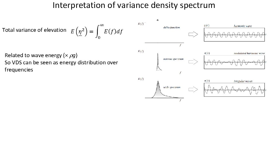
Interpretation of variance density spectrum Total variance of elevation Related to wave energy (× rg) So VDS can be seen as energy distribution over frequencies

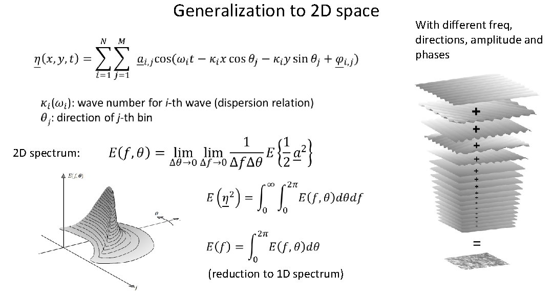
Generalization to 2 D space 2 D spectrum: (reduction to 1 D spectrum) With different freq, directions, amplitude and phases

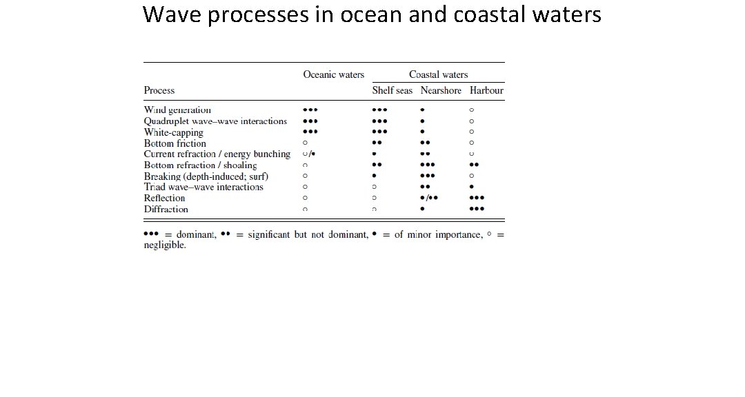
Wave processes in ocean and coastal waters

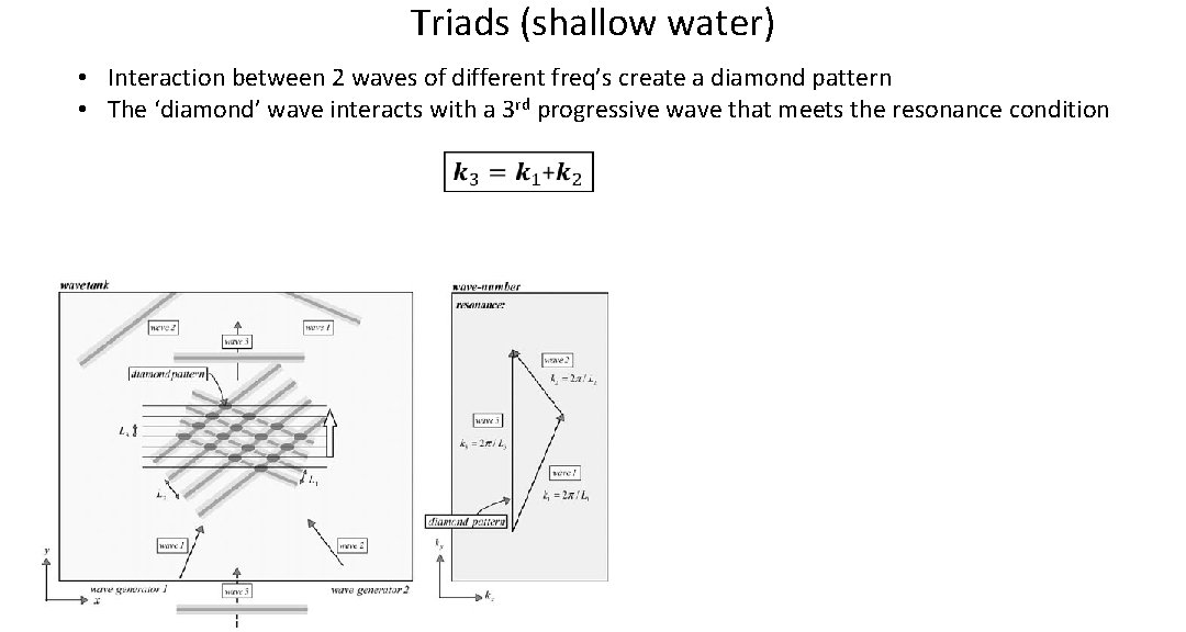
Triads (shallow water) • Interaction between 2 waves of different freq’s create a diamond pattern • The ‘diamond’ wave interacts with a 3 rd progressive wave that meets the resonance condition

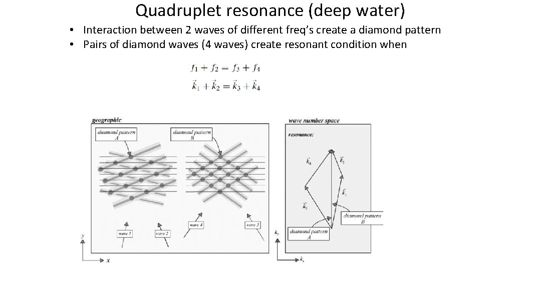
Quadruplet resonance (deep water) • Interaction between 2 waves of different freq’s create a diamond pattern • Pairs of diamond waves (4 waves) create resonant condition when

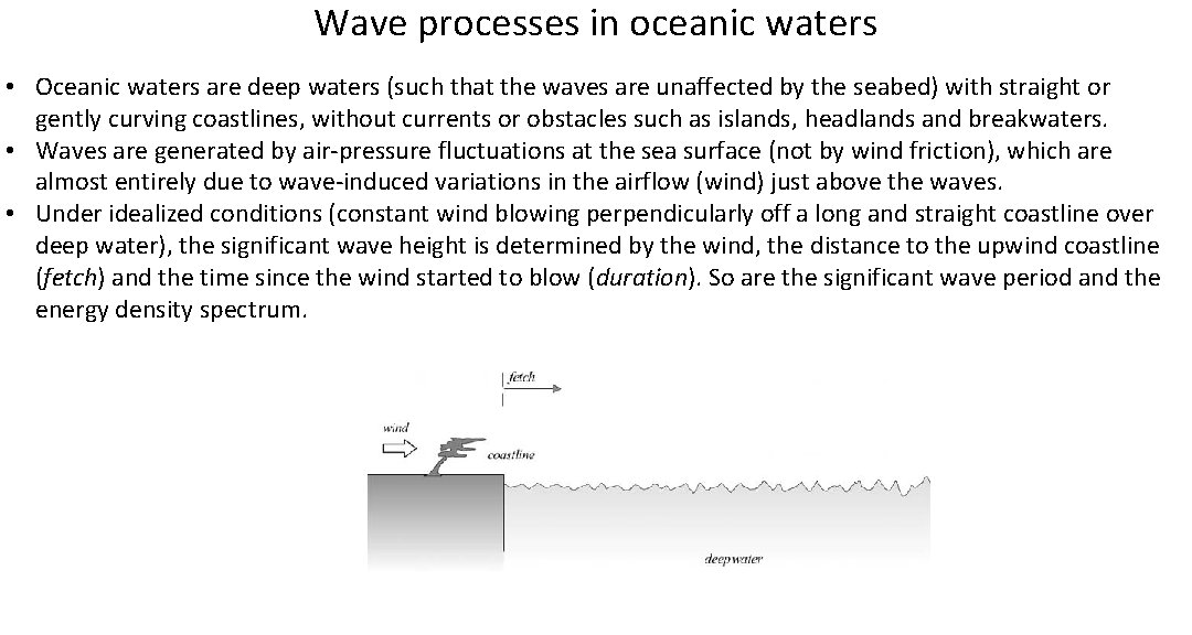
Wave processes in oceanic waters • Oceanic waters are deep waters (such that the waves are unaffected by the seabed) with straight or gently curving coastlines, without currents or obstacles such as islands, headlands and breakwaters. • Waves are generated by air-pressure fluctuations at the sea surface (not by wind friction), which are almost entirely due to wave-induced variations in the airflow (wind) just above the waves. • Under idealized conditions (constant wind blowing perpendicularly off a long and straight coastline over deep water), the significant wave height is determined by the wind, the distance to the upwind coastline (fetch) and the time since the wind started to blow (duration). So are the significant wave period and the energy density spectrum.

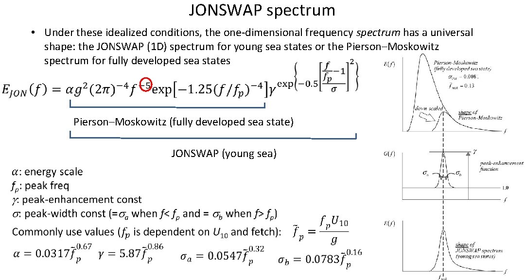
JONSWAP spectrum • Under these idealized conditions, the one-dimensional frequency spectrum has a universal shape: the JONSWAP (1 D) spectrum for young sea states or the Pierson–Moskowitz spectrum for fully developed sea states Pierson–Moskowitz (fully developed sea state) JONSWAP (young sea)

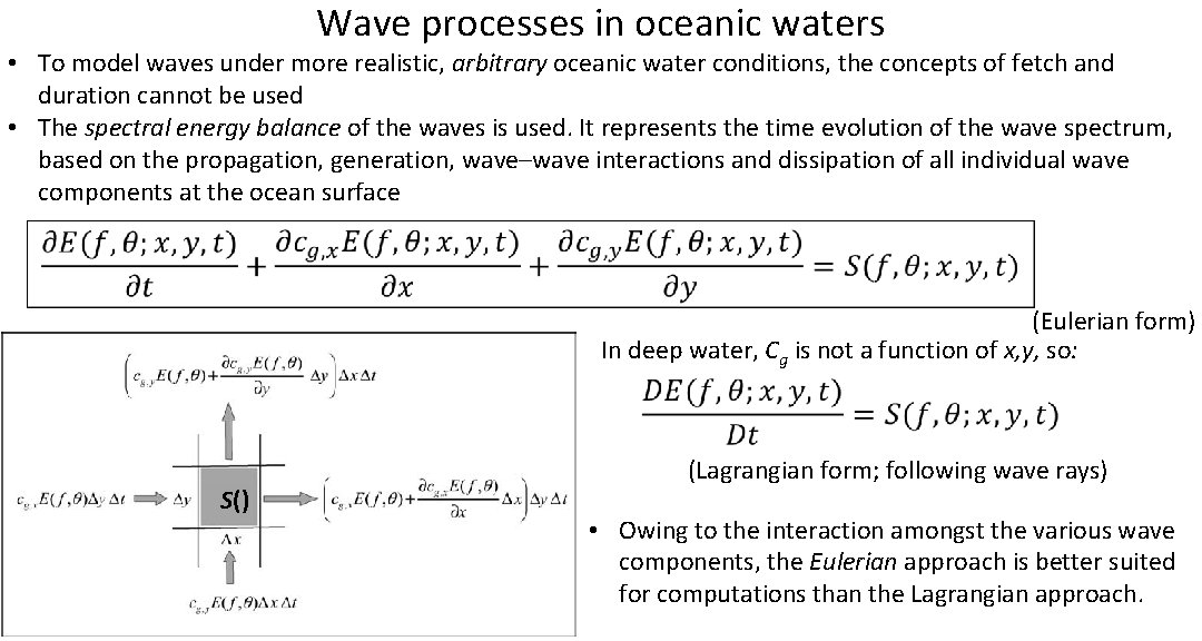
Wave processes in oceanic waters • To model waves under more realistic, arbitrary oceanic water conditions, the concepts of fetch and duration cannot be used • The spectral energy balance of the waves is used. It represents the time evolution of the wave spectrum, based on the propagation, generation, wave–wave interactions and dissipation of all individual wave components at the ocean surface (Eulerian form) In deep water, Cg is not a function of x, y, so: S() (Lagrangian form; following wave rays) • Owing to the interaction amongst the various wave components, the Eulerian approach is better suited for computations than the Lagrangian approach.

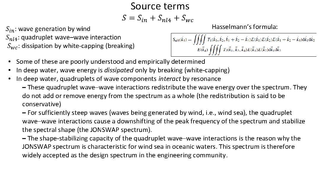
Source terms Hasselmann’s formula: • Some of these are poorly understood and empirically determined • In deep water, wave energy is dissipated only by breaking (white-capping) • In deep water, quadruplets of wave components interact by resonance – These quadruplet wave–wave interactions redistribute the wave energy over the spectrum. They do not add or remove energy from the spectrum as a whole (the redistribution is said to be conservative) – For sufficiently steep waves (waves being generated by wind, i. e. , wind sea), the quadruplet wave–wave interactions cause a downshifting of the peak frequency of the spectrum and stabilize the spectral shape (the JONSWAP spectrum). – The shape-stabilizing capacity of the quadruplet wave–wave interactions is the reason why the JONSWAP spectrum is characteristic for wind sea in oceanic waters. This spectrum is therefore widely accepted as the design spectrum in the engineering community.

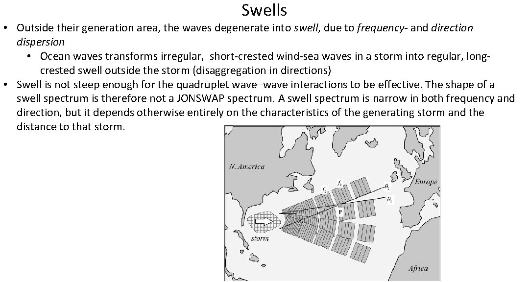
Swells • Outside their generation area, the waves degenerate into swell, due to frequency- and direction dispersion • Ocean waves transforms irregular, short-crested wind-sea waves in a storm into regular, longcrested swell outside the storm (disaggregation in directions) • Swell is not steep enough for the quadruplet wave–wave interactions to be effective. The shape of a swell spectrum is therefore not a JONSWAP spectrum. A swell spectrum is narrow in both frequency and direction, but it depends otherwise entirely on the characteristics of the generating storm and the distance to that storm.

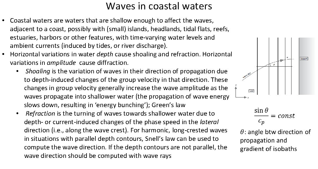
Waves in coastal waters • Coastal waters are waters that are shallow enough to affect the waves, adjacent to a coast, possibly with (small) islands, headlands, tidal flats, reefs, estuaries, harbors or other features, with time-varying water levels and ambient currents (induced by tides, or river discharge). • Horizontal variations in water depth cause shoaling and refraction. Horizontal variations in amplitude cause diffraction. • Shoaling is the variation of waves in their direction of propagation due to depth-induced changes of the group velocity in that direction. These changes in group velocity generally increase the wave amplitude as the waves propagate into shallower water (the propagation of wave energy slows down, resulting in ‘energy bunching’); Green’s law • Refraction is the turning of waves towards shallower water due to depth- or current-induced changes of the phase speed in the lateral direction (i. e. , along the wave crest). For harmonic, long-crested waves in situations with parallel depth contours, Snell’s law can be used to compute the wave direction. If the depth contours are not parallel, the wave direction should be computed with wave rays

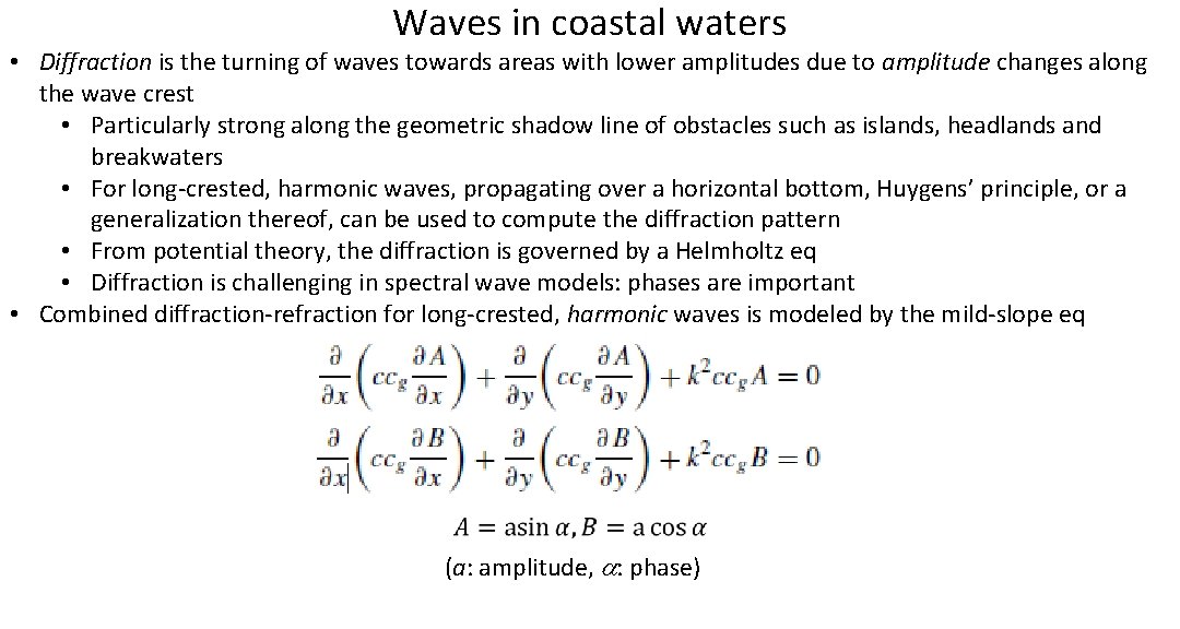
Waves in coastal waters • Diffraction is the turning of waves towards areas with lower amplitudes due to amplitude changes along the wave crest • Particularly strong along the geometric shadow line of obstacles such as islands, headlands and breakwaters • For long-crested, harmonic waves, propagating over a horizontal bottom, Huygens’ principle, or a generalization thereof, can be used to compute the diffraction pattern • From potential theory, the diffraction is governed by a Helmholtz eq • Diffraction is challenging in spectral wave models: phases are important • Combined diffraction-refraction for long-crested, harmonic waves is modeled by the mild-slope eq (a: amplitude, a: phase)

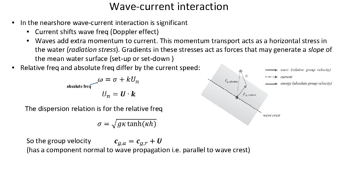
Wave-current interaction • In the nearshore wave-current interaction is significant • Current shifts wave freq (Doppler effect) • Waves add extra momentum to current. This momentum transport acts as a horizontal stress in the water (radiation stress). Gradients in these stresses act as forces that may generate a slope of the mean water surface (set-up or set-down ) • Relative freq and absolute freq differ by the current speed: absolute freq The dispersion relation is for the relative freq So the group velocity (has a component normal to wave propagation i. e. parallel to wave crest)

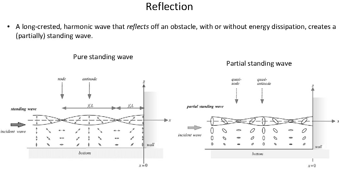
Reflection • A long-crested, harmonic wave that reflects off an obstacle, with or without energy dissipation, creates a (partially) standing wave. Pure standing wave Partial standing wave

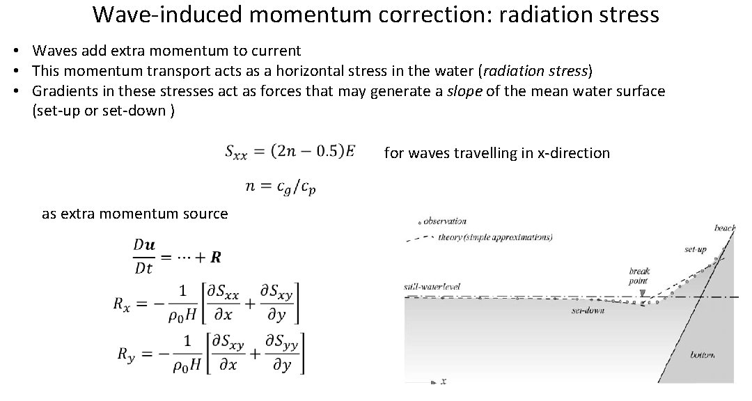
Wave-induced momentum correction: radiation stress • Waves add extra momentum to current • This momentum transport acts as a horizontal stress in the water (radiation stress) • Gradients in these stresses act as forces that may generate a slope of the mean water surface (set-up or set-down ) for waves travelling in x-direction as extra momentum source

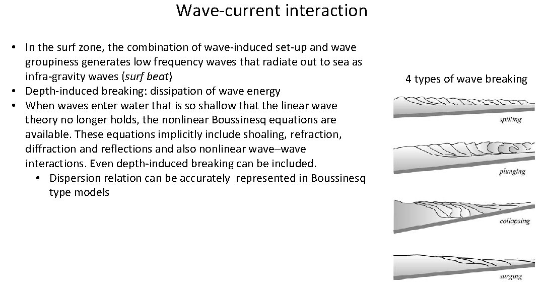
Wave-current interaction • In the surf zone, the combination of wave-induced set-up and wave groupiness generates low frequency waves that radiate out to sea as infra-gravity waves (surf beat) • Depth-induced breaking: dissipation of wave energy • When waves enter water that is so shallow that the linear wave theory no longer holds, the nonlinear Boussinesq equations are available. These equations implicitly include shoaling, refraction, diffraction and reflections and also nonlinear wave–wave interactions. Even depth-induced breaking can be included. • Dispersion relation can be accurately represented in Boussinesq type models 4 types of wave breaking

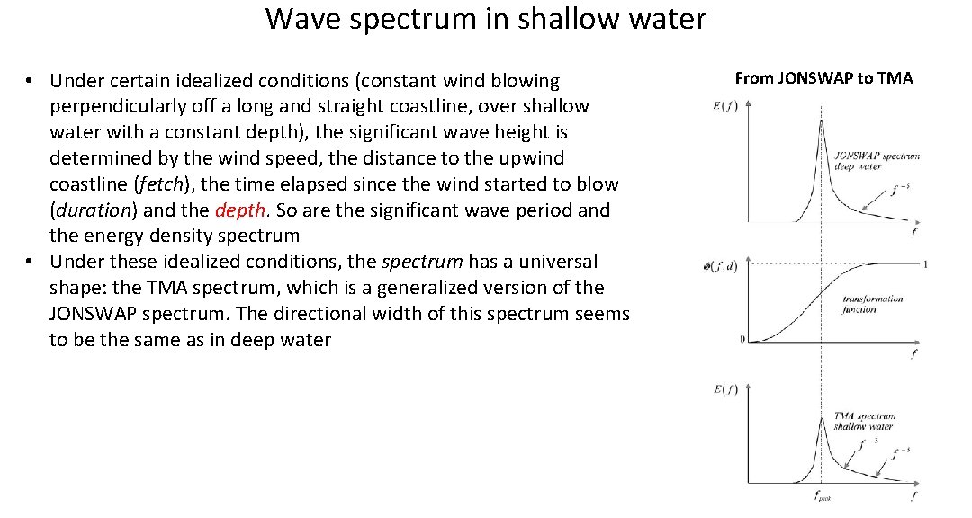
Wave spectrum in shallow water • Under certain idealized conditions (constant wind blowing perpendicularly off a long and straight coastline, over shallow water with a constant depth), the significant wave height is determined by the wind speed, the distance to the upwind coastline (fetch), the time elapsed since the wind started to blow (duration) and the depth. So are the significant wave period and the energy density spectrum • Under these idealized conditions, the spectrum has a universal shape: the TMA spectrum, which is a generalized version of the JONSWAP spectrum. The directional width of this spectrum seems to be the same as in deep water From JONSWAP to TMA

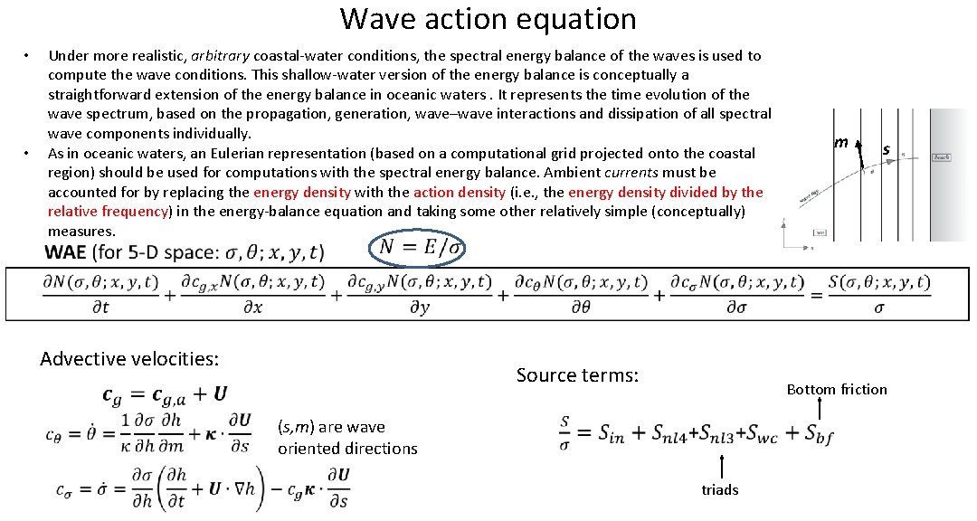
Wave action equation Under more realistic, arbitrary coastal-water conditions, the spectral energy balance of the waves is used to compute the wave conditions. This shallow-water version of the energy balance is conceptually a straightforward extension of the energy balance in oceanic waters. It represents the time evolution of the wave spectrum, based on the propagation, generation, wave–wave interactions and dissipation of all spectral wave components individually. As in oceanic waters, an Eulerian representation (based on a computational grid projected onto the coastal region) should be used for computations with the spectral energy balance. Ambient currents must be accounted for by replacing the energy density with the action density (i. e. , the energy density divided by the relative frequency) in the energy-balance equation and taking some other relatively simple (conceptually) measures. • • m s Advective velocities: Source terms: (s, m) are wave oriented directions Bottom friction triads

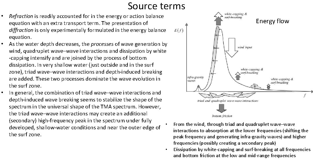
Source terms • Refraction is readily accounted for in the energy or action balance Energy flow equation with an extra transport term. The presentation of diffraction is only experimentally formulated in the energy balance equation. • As the water depth decreases, the processes of wave generation by wind, quadruplet wave–wave interactions and dissipation by white -capping intensify and are joined by the process of bottom dissipation. In very shallow water (just outside and in the surf zone), triad wave–wave interactions and depth-induced breaking are added. These two processes dominate the wave evolution in the surf zone. • In general, the combination of triad wave–wave interactions and depth-induced wave breaking seems to stabilize the shape of the spectrum in the universal shape of the TMA spectrum. However, the triad wave–wave interactions may create an additional (secondary) high-frequency peak in the spectrum under fully • From the wind, through triad and quadruplet wave–wave developed, shallow-water conditions and near the outer edge of interactions to absorption at the lower frequencies (shifting the surf zone. peak frequency and generating infra-gravity waves) and higher • frequencies (possibly creating a secondary peak) Dissipation by white-capping and surf-breaking at all frequencies and bottom friction at the low and mid-range frequencies

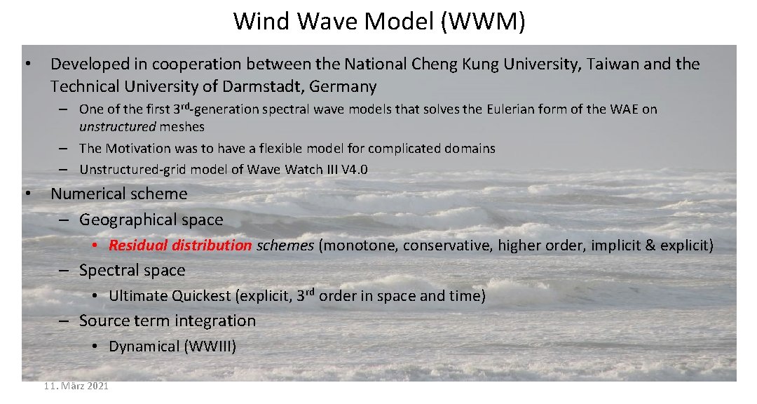
Wind Wave Model (WWM) • Developed in cooperation between the National Cheng Kung University, Taiwan and the Technical University of Darmstadt, Germany – One of the first 3 rd-generation spectral wave models that solves the Eulerian form of the WAE on unstructured meshes – The Motivation was to have a flexible model for complicated domains – Unstructured-grid model of Wave Watch III V 4. 0 • Numerical scheme – Geographical space • Residual distribution schemes (monotone, conservative, higher order, implicit & explicit) – Spectral space • Ultimate Quickest (explicit, 3 rd order in space and time) – Source term integration • Dynamical (WWIII) 11. März 2021

Wind Wave Model (WWM) • Physical formulation – Unified physics from deep to shallow water – The latest version of Fabrice Ardhuin’s of deep water physics – Extended WAE for strongly varying depths and wave-currents interactions; wave diffraction (Toledo et al. 2015, WISE 2010) • WWM fully coupled to SCHISM – Callable as a routine – Use same grid – efficiency – Both models are robust • Radiation stress formulations – Longuet-Higgins and Stewart (2 D) – Ardhuin’s vortex formalism

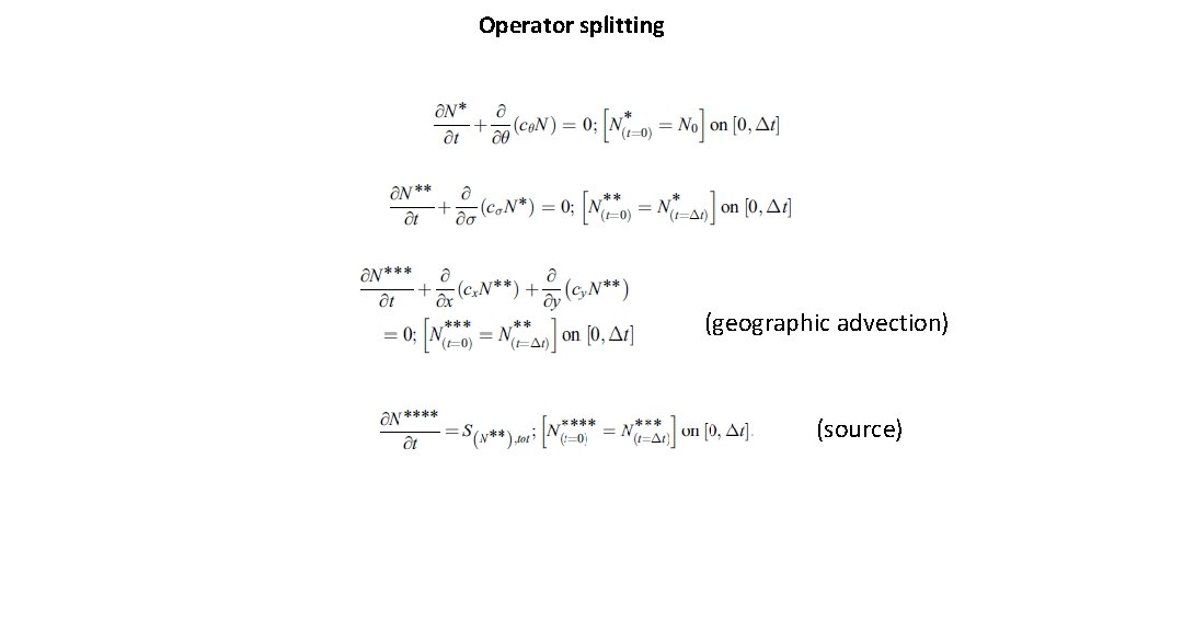
Operator splitting (geographic advection) (source)

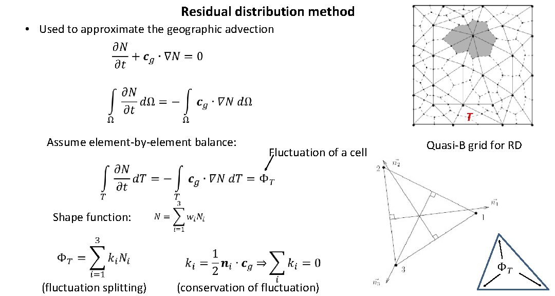
Residual distribution method • Used to approximate the geographic advection T Assume element-by-element balance: Shape function: Fluctuation of a cell Quasi-B grid for RD (fluctuation splitting) (conservation of fluctuation)

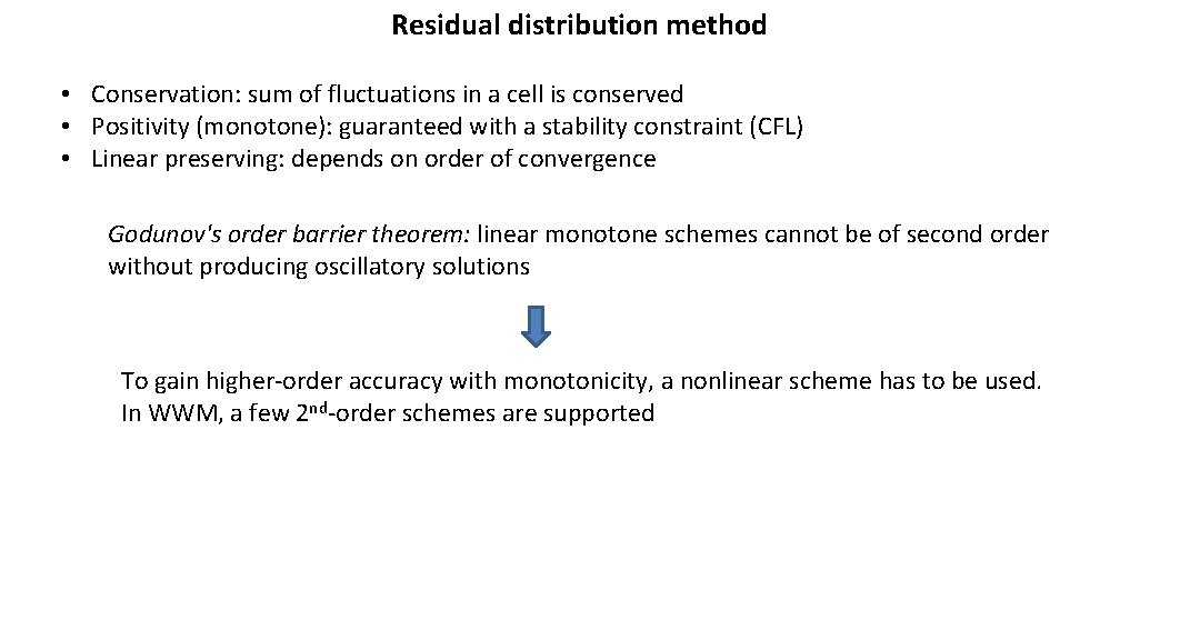
Residual distribution method • Conservation: sum of fluctuations in a cell is conserved • Positivity (monotone): guaranteed with a stability constraint (CFL) • Linear preserving: depends on order of convergence Godunov's order barrier theorem: linear monotone schemes cannot be of second order without producing oscillatory solutions To gain higher-order accuracy with monotonicity, a nonlinear scheme has to be used. In WWM, a few 2 nd-order schemes are supported

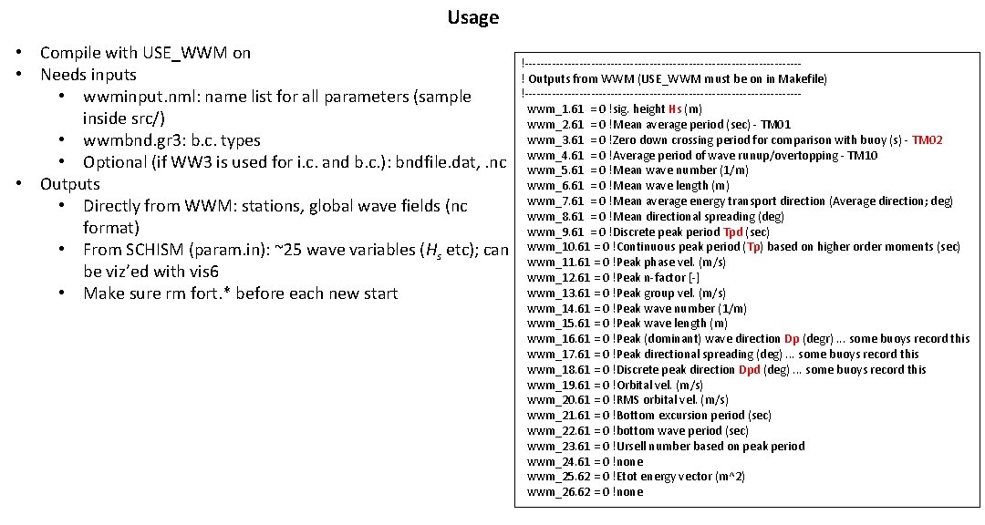
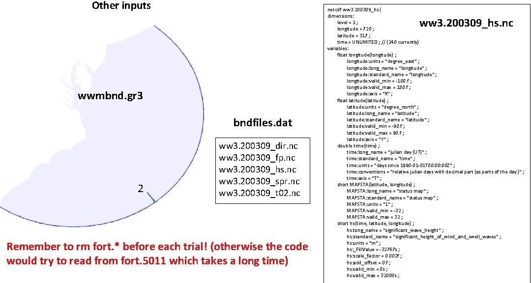
Usage • Compile with USE_WWM on • Needs inputs • wwminput. nml: name list for all parameters (sample inside src/) • wwmbnd. gr 3: b. c. types • Optional (if WW 3 is used for i. c. and b. c. ): bndfile. dat, . nc • Outputs • Directly from WWM: stations, global wave fields (nc format) • From SCHISM (param. in): ~25 wave variables (Hs etc); can be viz’ed with vis 6 • Make sure rm fort. * before each new start !-----------------------------------! Outputs from WWM (USE_WWM must be on in Makefile) !----------------------------------- wwm_1. 61 = 0 !sig. height Hs (m) wwm_2. 61 = 0 !Mean average period (sec) - TM 01 wwm_3. 61 = 0 !Zero down crossing period for comparison with buoy (s) - TM 02 wwm_4. 61 = 0 !Average period of wave runup/overtopping - TM 10 wwm_5. 61 = 0 !Mean wave number (1/m) wwm_6. 61 = 0 !Mean wave length (m) wwm_7. 61 = 0 !Mean average energy transport direction (Average direction; deg) wwm_8. 61 = 0 !Mean directional spreading (deg) wwm_9. 61 = 0 !Discrete peak period Tpd (sec) wwm_10. 61 = 0 !Continuous peak period (Tp) based on higher order moments (sec) wwm_11. 61 = 0 !Peak phase vel. (m/s) wwm_12. 61 = 0 !Peak n-factor [-] wwm_13. 61 = 0 !Peak group vel. (m/s) wwm_14. 61 = 0 !Peak wave number (1/m) wwm_15. 61 = 0 !Peak wave length (m) wwm_16. 61 = 0 !Peak (dominant) wave direction Dp (degr). . . some buoys record this wwm_17. 61 = 0 !Peak directional spreading (deg). . . some buoys record this wwm_18. 61 = 0 !Discrete peak direction Dpd (deg). . . some buoys record this wwm_19. 61 = 0 !Orbital vel. (m/s) wwm_20. 61 = 0 !RMS orbital vel. (m/s) wwm_21. 61 = 0 !Bottom excursion period (sec) wwm_22. 61 = 0 !bottom wave period (sec) wwm_23. 61 = 0 !Ursell number based on peak period wwm_24. 61 = 0 !none wwm_25. 62 = 0 !Etot energy vector (m^2) wwm_26. 62 = 0 !none

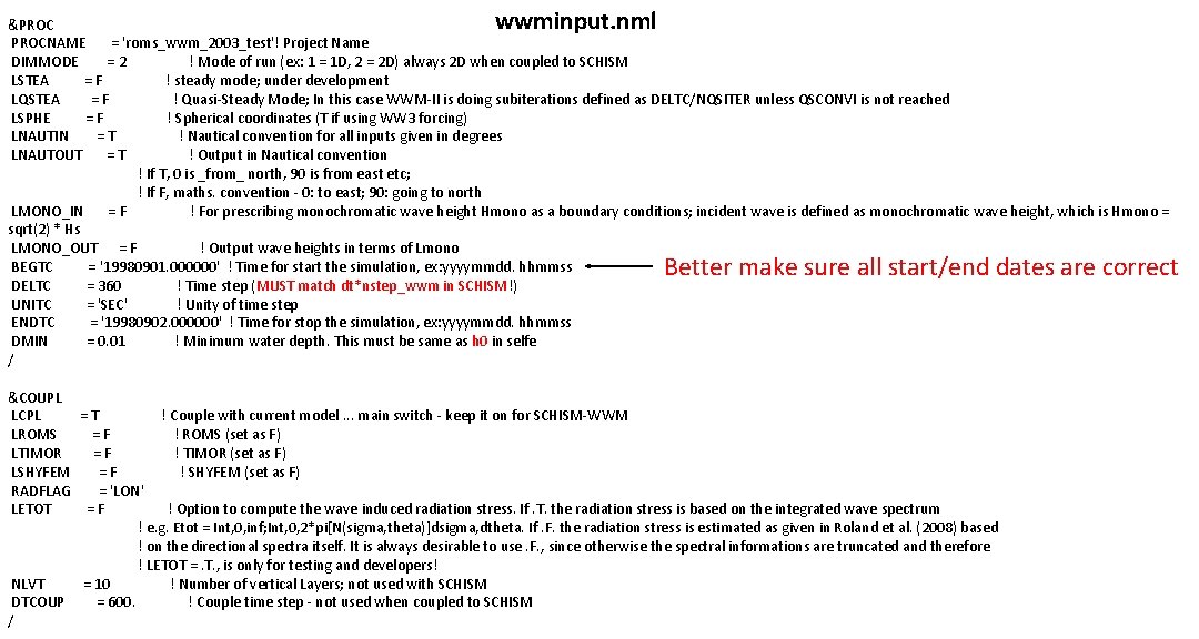
wwminput. nml &PROCNAME = 'roms_wwm_2003_test'! Project Name DIMMODE = 2 ! Mode of run (ex: 1 = 1 D, 2 = 2 D) always 2 D when coupled to SCHISM LSTEA = F ! steady mode; under development LQSTEA = F ! Quasi-Steady Mode; In this case WWM-II is doing subiterations defined as DELTC/NQSITER unless QSCONVI is not reached LSPHE = F ! Spherical coordinates (T if using WW 3 forcing) LNAUTIN = T ! Nautical convention for all inputs given in degrees LNAUTOUT = T ! Output in Nautical convention ! If T, 0 is _from_ north, 90 is from east etc; ! If F, maths. convention - 0: to east; 90: going to north LMONO_IN = F ! For prescribing monochromatic wave height Hmono as a boundary conditions; incident wave is defined as monochromatic wave height, which is Hmono = sqrt(2) * Hs LMONO_OUT = F ! Output wave heights in terms of Lmono BEGTC = '19980901. 000000' ! Time for start the simulation, ex: yyyymmdd. hhmmss DELTC = 360 ! Time step (MUST match dt*nstep_wwm in SCHISM!) UNITC = 'SEC' ! Unity of time step ENDTC = '19980902. 000000' ! Time for stop the simulation, ex: yyyymmdd. hhmmss DMIN = 0. 01 ! Minimum water depth. This must be same as h 0 in selfe / Better make sure all start/end dates are correct &COUPL LCPL = T ! Couple with current model. . . main switch - keep it on for SCHISM-WWM LROMS = F ! ROMS (set as F) LTIMOR = F ! TIMOR (set as F) LSHYFEM = F ! SHYFEM (set as F) RADFLAG = 'LON' LETOT = F ! Option to compute the wave induced radiation stress. If. T. the radiation stress is based on the integrated wave spectrum ! e. g. Etot = Int, 0, inf; Int, 0, 2*pi[N(sigma, theta)]dsigma, dtheta. If. F. the radiation stress is estimated as given in Roland et al. (2008) based ! on the directional spectra itself. It is always desirable to use. F. , since otherwise the spectral informations are truncated and therefore ! LETOT =. T. , is only for testing and developers! NLVT = 10 ! Number of vertical Layers; not used with SCHISM DTCOUP = 600. ! Couple time step - not used when coupled to SCHISM /

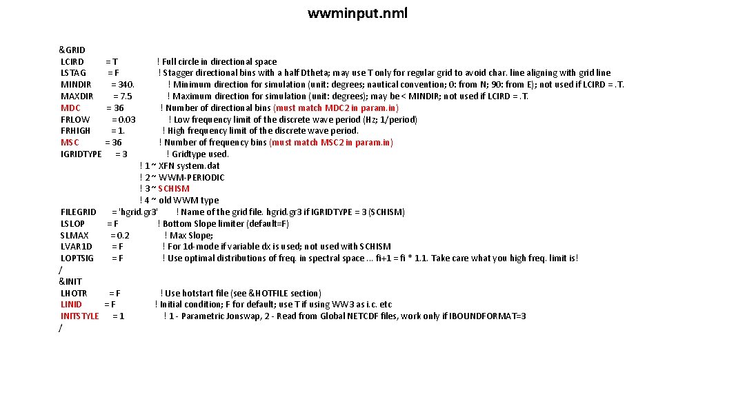
wwminput. nml &GRID LCIRD = T ! Full circle in directional space LSTAG = F ! Stagger directional bins with a half Dtheta; may use T only for regular grid to avoid char. line aligning with grid line MINDIR = 340. ! Minimum direction for simulation (unit: degrees; nautical convention; 0: from N; 90: from E); not used if LCIRD =. T. MAXDIR = 7. 5 ! Maximum direction for simulation (unit: degrees); may be < MINDIR; not used if LCIRD =. T. MDC = 36 ! Number of directional bins (must match MDC 2 in param. in) FRLOW = 0. 03 ! Low frequency limit of the discrete wave period (Hz; 1/period) FRHIGH = 1. ! High frequency limit of the discrete wave period. MSC = 36 ! Number of frequency bins (must match MSC 2 in param. in) IGRIDTYPE = 3 ! Gridtype used. ! 1 ~ XFN system. dat ! 2 ~ WWM-PERIODIC ! 3 ~ SCHISM ! 4 ~ old WWM type FILEGRID = 'hgrid. gr 3' ! Name of the grid file. hgrid. gr 3 if IGRIDTYPE = 3 (SCHISM) LSLOP = F ! Bottom Slope limiter (default=F) SLMAX = 0. 2 ! Max Slope; LVAR 1 D = F ! For 1 d-mode if variable dx is used; not used with SCHISM LOPTSIG = F ! Use optimal distributions of freq. in spectral space. . . fi+1 = fi * 1. 1. Take care what you high freq. limit is! / &INIT LHOTR = F ! Use hotstart file (see &HOTFILE section) LINID = F ! Initial condition; F for default; use T if using WW 3 as i. c. etc INITSTYLE = 1 ! 1 - Parametric Jonswap, 2 - Read from Global NETCDF files, work only if IBOUNDFORMAT=3 /

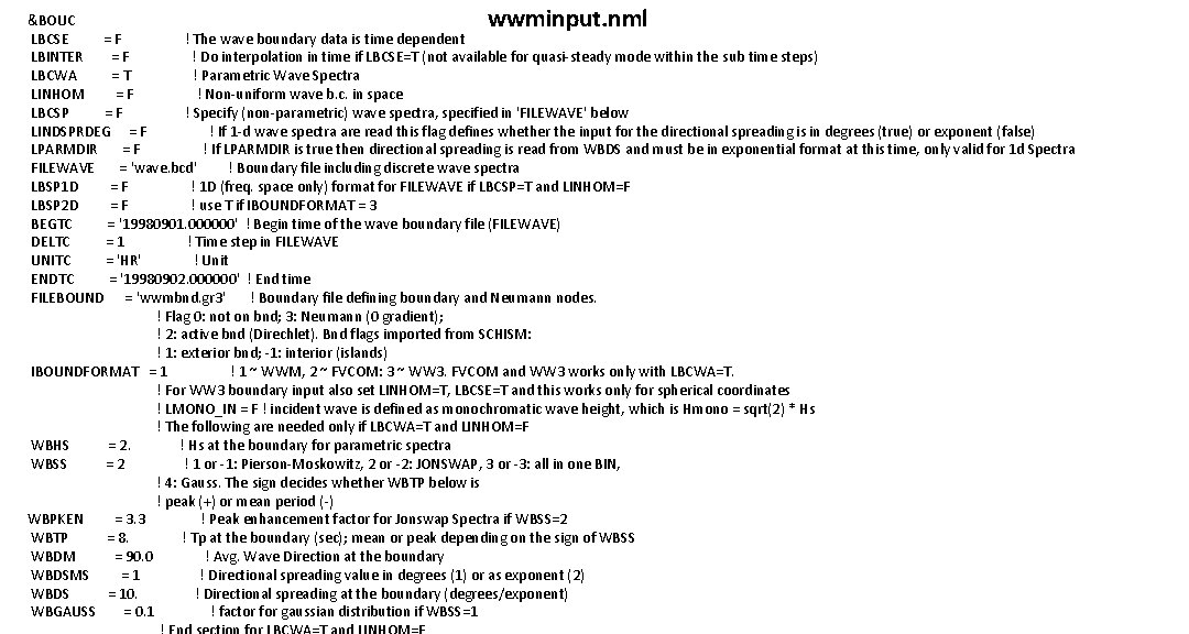
wwminput. nml &BOUC LBCSE = F ! The wave boundary data is time dependent LBINTER = F ! Do interpolation in time if LBCSE=T (not available for quasi-steady mode within the sub time steps) LBCWA = T ! Parametric Wave Spectra LINHOM = F ! Non-uniform wave b. c. in space LBCSP = F ! Specify (non-parametric) wave spectra, specified in 'FILEWAVE' below LINDSPRDEG = F ! If 1 -d wave spectra are read this flag defines whether the input for the directional spreading is in degrees (true) or exponent (false) LPARMDIR = F ! If LPARMDIR is true then directional spreading is read from WBDS and must be in exponential format at this time, only valid for 1 d Spectra FILEWAVE = 'wave. bcd' ! Boundary file including discrete wave spectra LBSP 1 D = F ! 1 D (freq. space only) format for FILEWAVE if LBCSP=T and LINHOM=F LBSP 2 D = F ! use T if IBOUNDFORMAT = 3 BEGTC = '19980901. 000000' ! Begin time of the wave boundary file (FILEWAVE) DELTC = 1 ! Time step in FILEWAVE UNITC = 'HR' ! Unit ENDTC = '19980902. 000000' ! End time FILEBOUND = 'wwmbnd. gr 3' ! Boundary file defining boundary and Neumann nodes. ! Flag 0: not on bnd; 3: Neumann (0 gradient); ! 2: active bnd (Direchlet). Bnd flags imported from SCHISM: ! 1: exterior bnd; -1: interior (islands) IBOUNDFORMAT = 1 ! 1 ~ WWM, 2 ~ FVCOM: 3 ~ WW 3. FVCOM and WW 3 works only with LBCWA=T. ! For WW 3 boundary input also set LINHOM=T, LBCSE=T and this works only for spherical coordinates ! LMONO_IN = F ! incident wave is defined as monochromatic wave height, which is Hmono = sqrt(2) * Hs ! The following are needed only if LBCWA=T and LINHOM=F WBHS = 2. ! Hs at the boundary for parametric spectra WBSS = 2 ! 1 or -1: Pierson-Moskowitz, 2 or -2: JONSWAP, 3 or -3: all in one BIN, ! 4: Gauss. The sign decides whether WBTP below is ! peak (+) or mean period (-) WBPKEN = 3. 3 ! Peak enhancement factor for Jonswap Spectra if WBSS=2 WBTP = 8. ! Tp at the boundary (sec); mean or peak depending on the sign of WBSS WBDM = 90. 0 ! Avg. Wave Direction at the boundary WBDSMS = 1 ! Directional spreading value in degrees (1) or as exponent (2) WBDS = 10. ! Directional spreading at the boundary (degrees/exponent) WBGAUSS = 0. 1 ! factor for gaussian distribution if WBSS=1

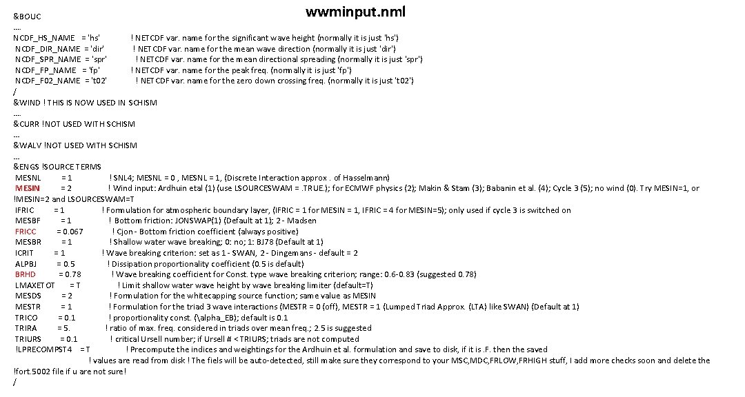
wwminput. nml &BOUC …. NCDF_HS_NAME = 'hs' ! NETCDF var. name for the significant wave height (normally it is just 'hs') NCDF_DIR_NAME = 'dir' ! NETCDF var. name for the mean wave direction (normally it is just 'dir') NCDF_SPR_NAME = 'spr' ! NETCDF var. name for the mean directional spreading (normally it is just 'spr') NCDF_FP_NAME = 'fp' ! NETCDF var. name for the peak freq. (normally it is just 'fp') NCDF_F 02_NAME = 't 02' ! NETCDF var. name for the zero down crossing freq. (normally it is just 't 02') / &WIND ! THIS IS NOW USED IN SCHISM …. &CURR !NOT USED WITH SCHISM … &WALV !NOT USED WITH SCHISM … &ENGS !SOURCE TERMS MESNL = 1 ! SNL 4; MESNL = 0 , MESNL = 1, (Discrete Interaction approx. of Hasselmann) MESIN = 2 ! Wind input: Ardhuin etal (1) (use LSOURCESWAM =. TRUE. ); for ECMWF physics (2); Makin & Stam (3); Babanin et al. (4); Cycle 3 (5); no wind (0). Try MESIN=1, or !MESIN=2 and LSOURCESWAM=T IFRIC = 1 ! Formulation for atmospheric boundary layer, (IFRIC = 1 for MESIN = 1, IFRIC = 4 for MESIN=5); only used if cycle 3 is switched on MESBF = 1 ! Bottom friction: JONSWAP(1) (Default at 1); 2 - Madsen FRICC = 0. 067 ! Cjon - Bottom friction coefficient (always positive) MESBR = 1 ! Shallow water wave breaking; 0: no; 1: BJ 78 (Default at 1) ICRIT = 1 ! Wave breaking criterion: set as 1 - SWAN, 2 - Dingemans - default = 2 ALPBJ = 0. 5 ! Dissipation proportionality coefficient (0. 5 is default) BRHD = 0. 78 ! Wave breaking coefficient for Const. type wave breaking criterion; range: 0. 6 -0. 83 (suggested 0. 78) LMAXETOT = T ! Limit shallow water wave height by wave breaking limiter (default=T) MESDS = 2 ! Formulation for the whitecapping source function; same value as MESIN MESTR = 1 ! Formulation for the triad 3 wave interactions (MESTR = 0 (off), MESTR = 1 (Lumped Triad Approx. (LTA) like SWAN) (Default at 1) TRICO = 0. 1 ! proportionality const. (alpha_EB); default is 0. 1 TRIRA = 5. ! ratio of max. freq. considered in triads over mean freq. ; 2. 5 is suggested TRIURS = 0. 1 ! critical Ursell number; if Ursell # < TRIURS; triads are not computed !LPRECOMPST 4 = T ! Precompute the indices and weightings for the Ardhuin et al. formulation and save to disk, if it is. F. then the saved ! values are read from disk ! The fiels will be auto-detected, still make sure they correspond to your MSC, MDC, FRLOW, FRHIGH stuff, I add more checks soon and delete the !fort. 5002 file if u are not sure! /

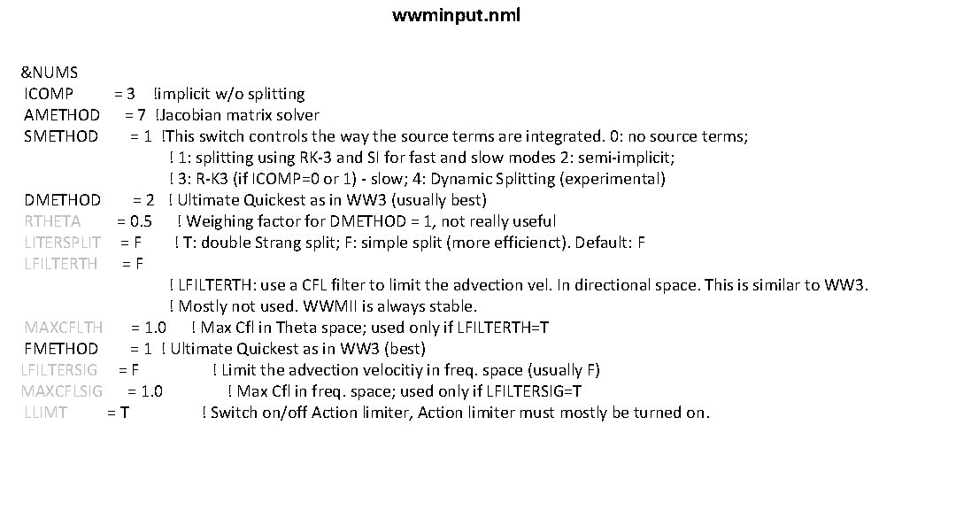
wwminput. nml &NUMS ICOMP = 3 !implicit w/o splitting AMETHOD = 7 !Jacobian matrix solver SMETHOD = 1 !This switch controls the way the source terms are integrated. 0: no source terms; ! 1: splitting using RK-3 and SI for fast and slow modes 2: semi-implicit; ! 3: R-K 3 (if ICOMP=0 or 1) - slow; 4: Dynamic Splitting (experimental) DMETHOD = 2 ! Ultimate Quickest as in WW 3 (usually best) RTHETA = 0. 5 ! Weighing factor for DMETHOD = 1, not really useful LITERSPLIT = F ! T: double Strang split; F: simple split (more efficienct). Default: F LFILTERTH = F ! LFILTERTH: use a CFL filter to limit the advection vel. In directional space. This is similar to WW 3. ! Mostly not used. WWMII is always stable. MAXCFLTH = 1. 0 ! Max Cfl in Theta space; used only if LFILTERTH=T FMETHOD = 1 ! Ultimate Quickest as in WW 3 (best) LFILTERSIG = F ! Limit the advection velocitiy in freq. space (usually F) MAXCFLSIG = 1. 0 ! Max Cfl in freq. space; used only if LFILTERSIG=T LLIMT = T ! Switch on/off Action limiter, Action limiter must mostly be turned on.

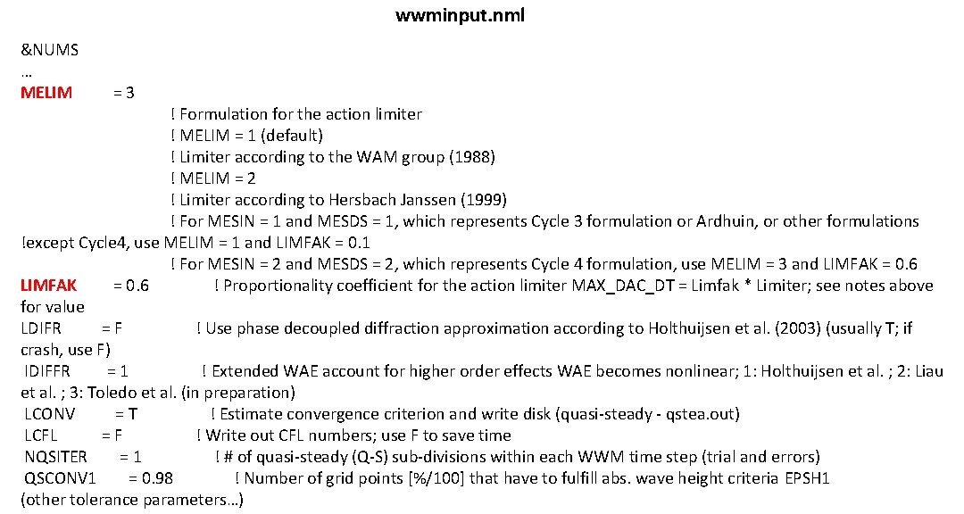
wwminput. nml &NUMS … MELIM = 3 ! Formulation for the action limiter ! MELIM = 1 (default) ! Limiter according to the WAM group (1988) ! MELIM = 2 ! Limiter according to Hersbach Janssen (1999) ! For MESIN = 1 and MESDS = 1, which represents Cycle 3 formulation or Ardhuin, or other formulations !except Cycle 4, use MELIM = 1 and LIMFAK = 0. 1 ! For MESIN = 2 and MESDS = 2, which represents Cycle 4 formulation, use MELIM = 3 and LIMFAK = 0. 6 LIMFAK = 0. 6 ! Proportionality coefficient for the action limiter MAX_DAC_DT = Limfak * Limiter; see notes above for value LDIFR = F ! Use phase decoupled diffraction approximation according to Holthuijsen et al. (2003) (usually T; if crash, use F) IDIFFR = 1 ! Extended WAE account for higher order effects WAE becomes nonlinear; 1: Holthuijsen et al. ; 2: Liau et al. ; 3: Toledo et al. (in preparation) LCONV = T ! Estimate convergence criterion and write disk (quasi-steady - qstea. out) LCFL = F ! Write out CFL numbers; use F to save time NQSITER = 1 ! # of quasi-steady (Q-S) sub-divisions within each WWM time step (trial and errors) QSCONV 1 = 0. 98 ! Number of grid points [%/100] that have to fulfill abs. wave height criteria EPSH 1 (other tolerance parameters…)

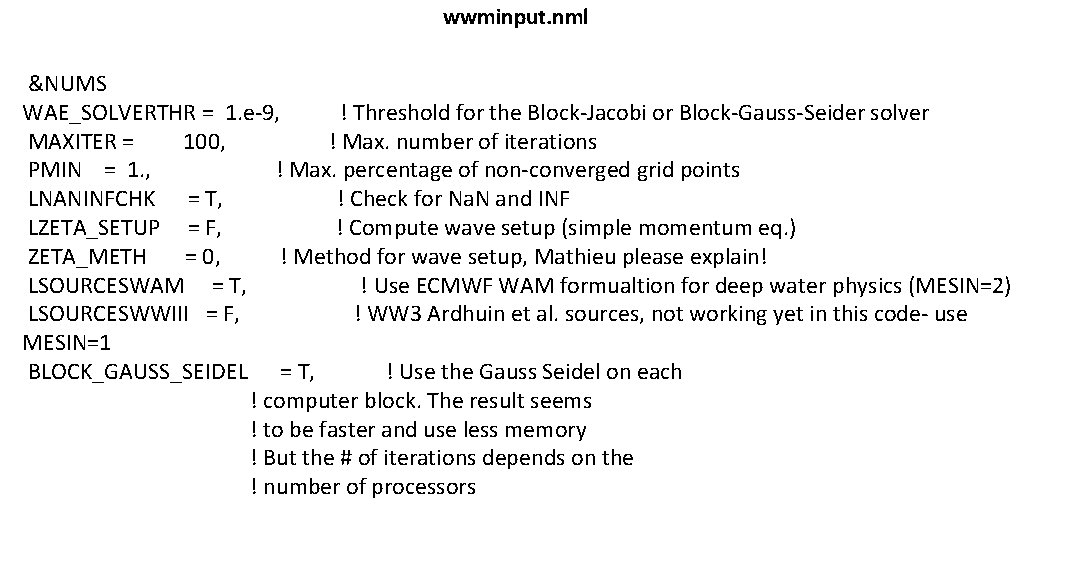
wwminput. nml &NUMS WAE_SOLVERTHR = 1. e-9, ! Threshold for the Block-Jacobi or Block-Gauss-Seider solver MAXITER = 100, ! Max. number of iterations PMIN = 1. , ! Max. percentage of non-converged grid points LNANINFCHK = T, ! Check for Na. N and INF LZETA_SETUP = F, ! Compute wave setup (simple momentum eq. ) ZETA_METH = 0, ! Method for wave setup, Mathieu please explain! LSOURCESWAM = T, ! Use ECMWF WAM formualtion for deep water physics (MESIN=2) LSOURCESWWIII = F, ! WW 3 Ardhuin et al. sources, not working yet in this code- use MESIN=1 BLOCK_GAUSS_SEIDEL = T, ! Use the Gauss Seidel on each ! computer block. The result seems ! to be faster and use less memory ! But the # of iterations depends on the ! number of processors

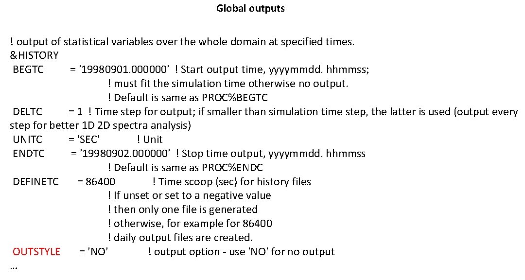
Global outputs ! output of statistical variables over the whole domain at specified times. &HISTORY BEGTC = '19980901. 000000' ! Start output time, yyyymmdd. hhmmss; ! must fit the simulation time otherwise no output. ! Default is same as PROC%BEGTC DELTC = 1 ! Time step for output; if smaller than simulation time step, the latter is used (output every step for better 1 D 2 D spectra analysis) UNITC = 'SEC' ! Unit ENDTC = '19980902. 000000' ! Stop time output, yyyymmdd. hhmmss ! Default is same as PROC%ENDC DEFINETC = 86400 ! Time scoop (sec) for history files ! If unset or set to a negative value ! then only one file is generated ! otherwise, for example for 86400 ! daily output files are created. OUTSTYLE = 'NO' ! output option - use 'NO' for no output …

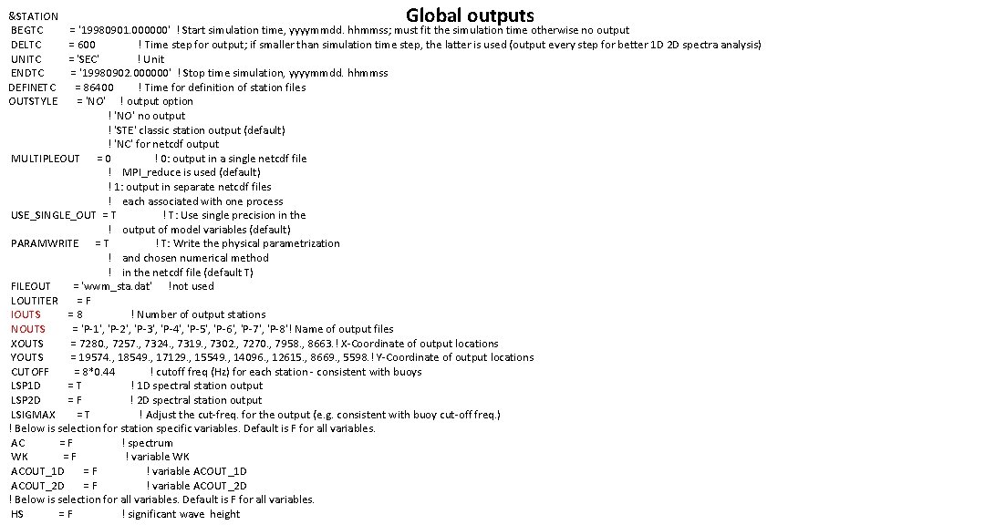
Global outputs &STATION BEGTC = '19980901. 000000' ! Start simulation time, yyyymmdd. hhmmss; must fit the simulation time otherwise no output DELTC = 600 ! Time step for output; if smaller than simulation time step, the latter is used (output every step for better 1 D 2 D spectra analysis) UNITC = 'SEC' ! Unit ENDTC = '19980902. 000000' ! Stop time simulation, yyyymmdd. hhmmss DEFINETC = 86400 ! Time for definition of station files OUTSTYLE = 'NO' ! output option ! 'NO' no output ! 'STE' classic station output (default) ! 'NC' for netcdf output MULTIPLEOUT = 0 ! 0: output in a single netcdf file ! MPI_reduce is used (default) ! 1: output in separate netcdf files ! each associated with one process USE_SINGLE_OUT = T ! T: Use single precision in the ! output of model variables (default) PARAMWRITE = T ! T: Write the physical parametrization ! and chosen numerical method ! in the netcdf file (default T) FILEOUT = 'wwm_sta. dat' !not used LOUTITER = F IOUTS = 8 ! Number of output stations NOUTS = 'P-1', 'P-2', 'P-3', 'P-4', 'P-5', 'P-6', 'P-7', 'P-8'! Name of output files XOUTS = 7280. , 7257. , 7324. , 7319. , 7302. , 7270. , 7958. , 8663. ! X-Coordinate of output locations YOUTS = 19574. , 18549. , 17129. , 15549. , 14096. , 12615. , 8669. , 5598. ! Y-Coordinate of output locations CUTOFF = 8*0. 44 ! cutoff freq (Hz) for each station - consistent with buoys LSP 1 D = T ! 1 D spectral station output LSP 2 D = F ! 2 D spectral station output LSIGMAX = T ! Adjust the cut-freq. for the output (e. g. consistent with buoy cut-off freq. ) ! Below is selection for station specific variables. Default is F for all variables. AC = F ! spectrum WK = F ! variable WK ACOUT_1 D = F ! variable ACOUT_1 D ACOUT_2 D = F ! variable ACOUT_2 D ! Below is selection for all variables. Default is F for all variables. HS = F ! significant wave height

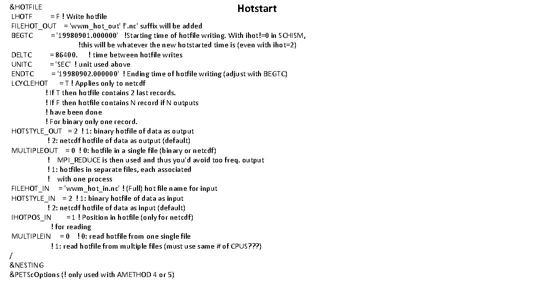
&HOTFILE Hotstart LHOTF = F ! Write hotfile FILEHOT_OUT = 'wwm_hot_out' !'. nc' suffix will be added BEGTC = '19980901. 000000' !Starting time of hotfile writing. With ihot!=0 in SCHISM, !this will be whatever the new hotstarted time is (even with ihot=2) DELTC = 86400. ! time between hotfile writes UNITC = 'SEC' ! unit used above ENDTC = '19980902. 000000' ! Ending time of hotfile writing (adjust with BEGTC) LCYCLEHOT = T ! Applies only to netcdf ! If T then hotfile contains 2 last records. ! If F then hotfile contains N record if N outputs ! have been done ! For binary only one record. HOTSTYLE_OUT = 2 ! 1: binary hotfile of data as output ! 2: netcdf hotfile of data as output (default) MULTIPLEOUT = 0 ! 0: hotfile in a single file (binary or netcdf) ! MPI_REDUCE is then used and thus you'd avoid too freq. output ! 1: hotfiles in separate files, each associated ! with one process FILEHOT_IN = 'wwm_hot_in. nc' ! (Full) hot file name for input HOTSTYLE_IN = 2 ! 1: binary hotfile of data as input ! 2: netcdf hotfile of data as input (default) IHOTPOS_IN = 1 ! Position in hotfile (only for netcdf) ! for reading MULTIPLEIN = 0 ! 0: read hotfile from one single file ! 1: read hotfile from multiple files (must use same # of CPUS? ? ? ) / &NESTING &PETSc. Options (! only used with AMETHOD 4 or 5)

Other inputs netcdf ww 3. 200309_hs { dimensions: level = 1 ; longitude = 720 ; latitude = 317 ; time = UNLIMITED ; // (240 currently) variables: float longitude(longitude) ; longitude: units = "degree_east" ; longitude: long_name = "longitude" ; longitude: standard_name = "longitude" ; longitude: valid_min = -180. f ; longitude: valid_max = 180. f ; longitude: axis = "X" ; float latitude(latitude) ; latitude: units = "degree_north" ; latitude: long_name = "latitude" ; latitude: standard_name = "latitude" ; latitude: valid_min = -90. f ; latitude: valid_max = 90. f ; latitude: axis = "Y" ; double time(time) ; time: long_name = "julian day (UT)" ; time: standard_name = "time" ; time: units = "days since 1990 -01 -01 T 00: 00 Z" ; time: conventions = "relative julian days with decimal part (as parts of the day )" ; time: axis = "T" ; short MAPSTA(latitude, longitude) ; MAPSTA: long_name = "status map" ; MAPSTA: standard_name = "status map" ; MAPSTA: units = "1" ; MAPSTA: valid_min = -32 ; MAPSTA: valid_max = 32 ; short hs(time, latitude, longitude) ; hs: long_name = "significant_wave_height" ; hs: standard_name = "significant_height_of_wind_and_swell_waves" ; hs: units = "m" ; hs: _Fill. Value = -32767 s ; hs: scale_factor = 0. 002 f ; hs: add_offset = 0. f ; hs: valid_min = 0 s ; hs: valid_max = 32000 s ; ww 3. 200309_hs. nc wwmbnd. gr 3 bndfiles. dat 2 ww 3. 200309_dir. nc ww 3. 200309_fp. nc ww 3. 200309_hs. nc ww 3. 200309_spr. nc ww 3. 200309_t 02. nc Remember to rm fort. * before each trial! (otherwise the code would try to read from fort. 5011 which takes a long time)

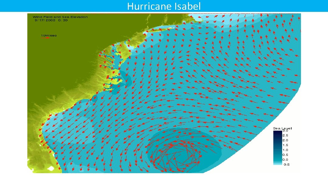
Hurricane Isabel

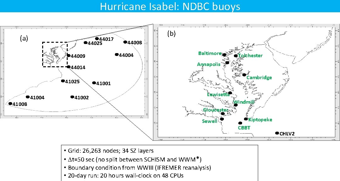
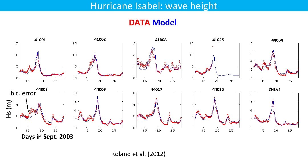
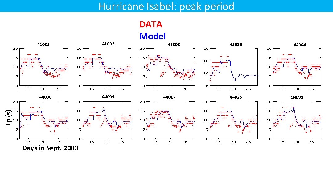
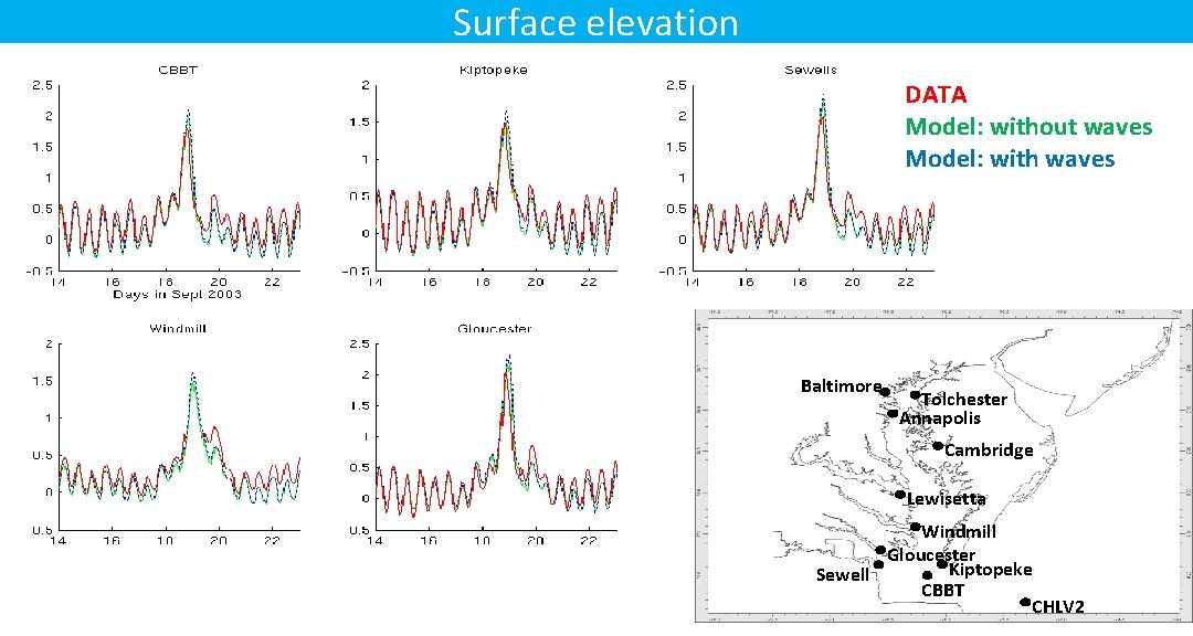
Hurricane Isabel: NDBC buoys (a) 44017 44025 41008 41002 Baltimore Tolchester Annapolis 44014 41004 44008 44004 44009 41025 (b) Cambridge 41001 Lewisetta Windmill Gloucester Sewell • Grid: 26, 263 nodes; 34 SZ layers • Dt=50 sec (no split between SCHISM and WWM*) • Boundary condition from WWIII (IFREMER reanalysis) • 20 -day run: 20 hours wall-clock on 48 CPUs Kiptopeke CBBT CHLV 2

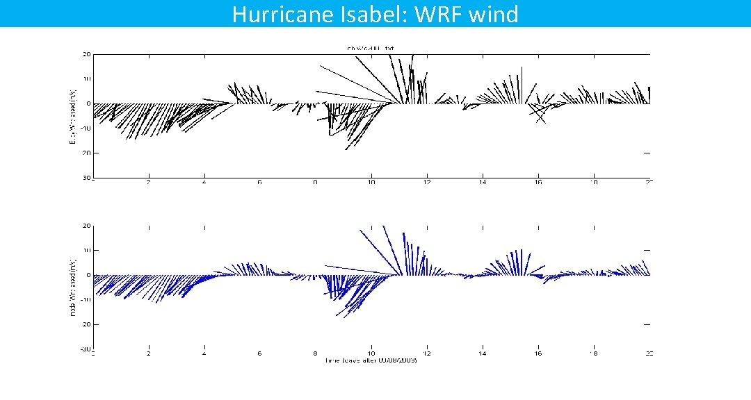
Hurricane Isabel: WRF wind

Hurricane Isabel: wave height DATA Model 41001 44009 41008 44017 Hs (m) b. c. error 44008 41002 Days in Sept. 2003 Roland et al. (2012) 41025 44004 CHLV 2

Hurricane Isabel: peak period 41001 Tp (s) 44008 Days in Sept. 2003 41002 44009 DATA Model 41008 44017 41025 44004 CHLV 2

Surface elevation DATA Model: without waves Model: with waves Baltimore Tolchester Annapolis Cambridge Lewisetta Windmill Gloucester Kiptopeke Sewell CBBT CHLV 2

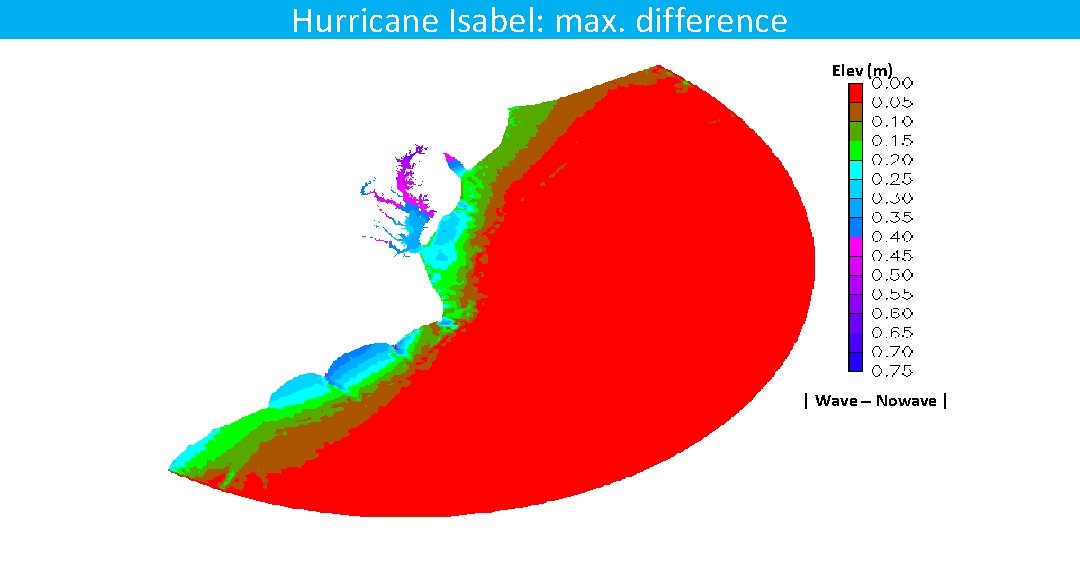
Hurricane Isabel: max. difference Elev (m) | Wave - Nowave |

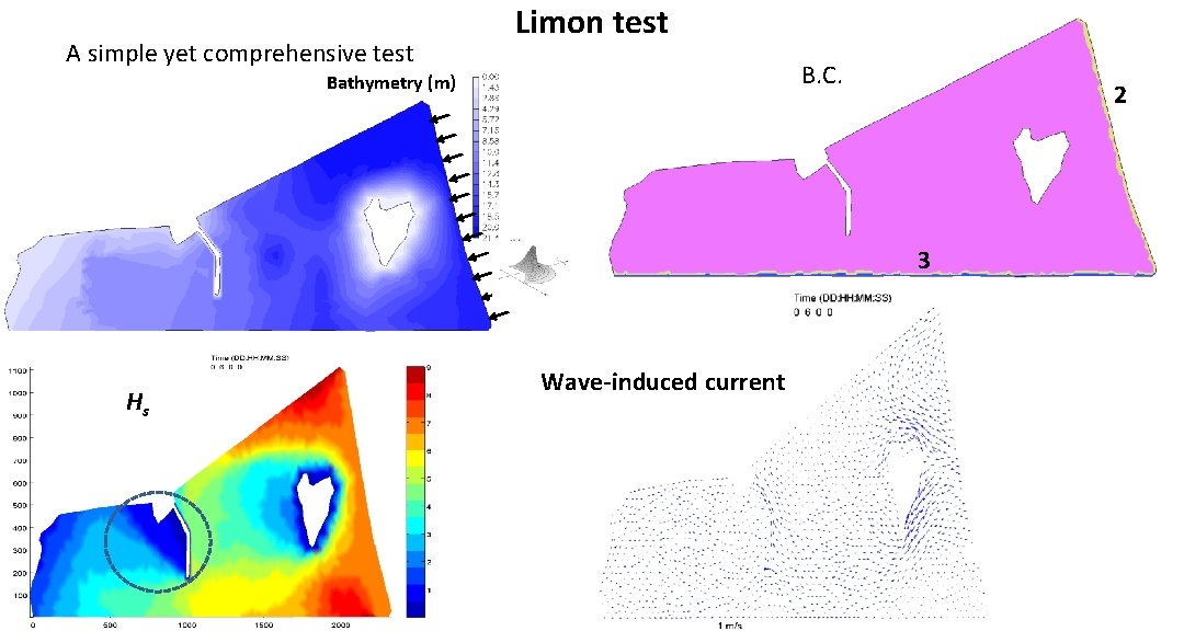
A simple yet comprehensive test Limon test B. C. Bathymetry (m) 2 3 Hs Wave-induced current

Wave-sediment exercises Training_Course_Cases/ 1) SCHISM-WWM-SED 3 D: Ches Bay with wave and sediment transport – need to upgrade to latest version 2) meander_RUN 02 h: sediment transport only; migration of channel due to morphodynamics