Scheduling Algorithms 4541 633 A So C Design

Scheduling Algorithms 4541. 633 A So. C Design Automation School of EECS Seoul National University

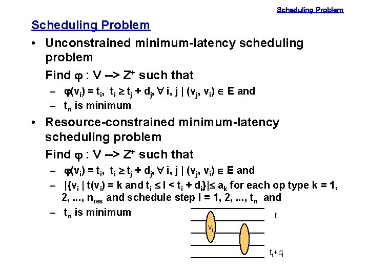
Scheduling Problem • Unconstrained minimum-latency scheduling problem Find j : V --> Z+ such that – j(vi) = ti, ti ³ tj + dj, " i, j | (vj, vi) Î E and – tn is minimum • Resource-constrained minimum-latency scheduling problem Find j : V --> Z+ such that – j(vi) = ti, ti ³ tj + dj, " i, j | (vj, vi) Î E and – |{vi | t(vi) = k and ti £ l < ti + di}|£ ak for each op type k = 1, 2, . . . , nres and schedule step l = 1, 2, . . . , tn and – tn is minimum ti vi ti+di

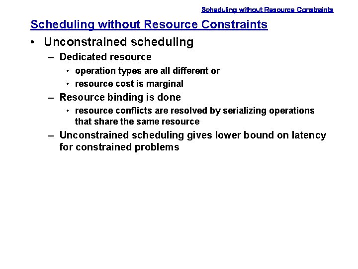
Scheduling without Resource Constraints • Unconstrained scheduling – Dedicated resource • operation types are all different or • resource cost is marginal – Resource binding is done • resource conflicts are resolved by serializing operations that share the same resource – Unconstrained scheduling gives lower bound on latency for constrained problems

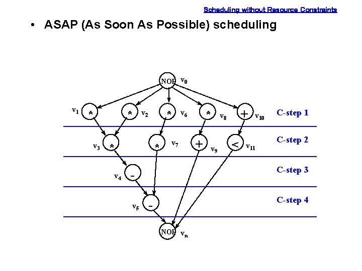
Scheduling without Resource Constraints • ASAP (As Soon As Possible) scheduling NOP v 0 v 1 * v 3 * * v 2 * v 4 * v 7 + v 9 + v 8 < v 10 v 11 C-step 2 C-step 3 v 5 * v 6 C-step 4 NOP vn

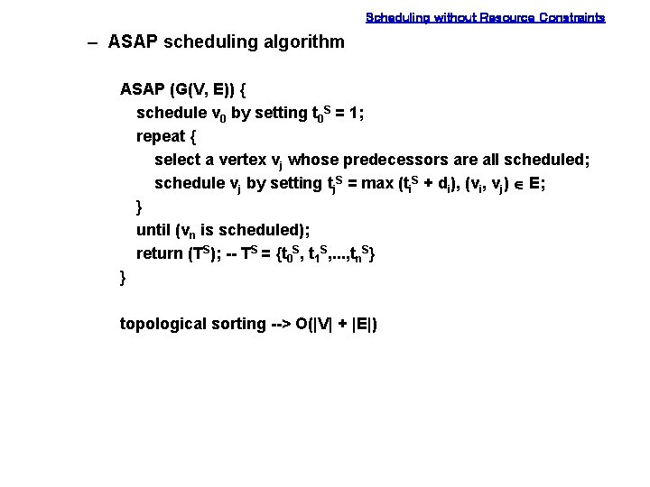
Scheduling without Resource Constraints – ASAP scheduling algorithm ASAP (G(V, E)) { schedule v 0 by setting t 0 S = 1; repeat { select a vertex vj whose predecessors are all scheduled; schedule vj by setting tj. S = max (ti. S + di), (vi, vj) Î E; } until (vn is scheduled); return (TS); -- TS = {t 0 S, t 1 S, . . . , tn. S} } topological sorting --> O(|V| + |E|)

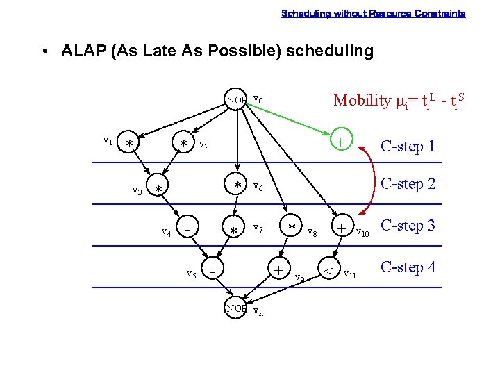
Scheduling without Resource Constraints • ALAP (As Late As Possible) scheduling Mobility mi= ti. L - ti. S NOP v 0 v 1 * v 3 * + v 2 * * v 4 v 5 * C-step 1 C-step 2 v 6 * v 7 - + NOP vn v 9 + v 8 < v 10 v 11 C-step 3 C-step 4

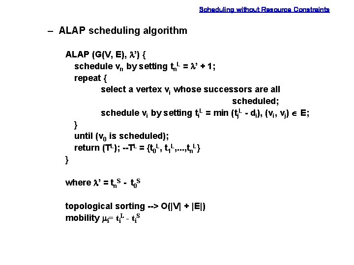
Scheduling without Resource Constraints – ALAP scheduling algorithm ALAP (G(V, E), l’) { schedule vn by setting tn. L = l’ + 1; repeat { select a vertex vi whose successors are all scheduled; schedule vi by setting ti. L = min (tj. L - di), (vi, vj) Î E; } until (v 0 is scheduled); return (TL); --TL = {t 0 L, t 1 L, . . . , tn. L} } where l’ = tn. S - t 0 S topological sorting --> O(|V| + |E|) mobility mi= ti. L - ti. S

Scheduling with Resource Constraints • Given resource constraint find area/latency tradeoff points • Integer Linear Programming (ILP) model – C. -T. Hwang, J. -H. Lee, and Y. -C. Hsu, “A formal approach to the scheduling problem in high level synthesis, ” IEEE Trans. on CAD, April 1991. – Exact solution but NP-complete

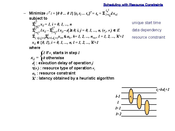
Scheduling with Resource Constraints tn. L – Minimize t = [0 0. . . 0 1] [t 0 t 1. . . tn = S l=t Sl xnl n subject to ti. L Sl=t S xil = 1, i = 0, 1, . . . , n c. T ti. L i S S l=ti l xil – ]T tj. L Sl=t S j l xjl - dj ³ 0, i, j = 0, 1, . . . , n, (vj , vi) Î E l S i: t(v )=k. Sm=l-d +1 xim £ ak , k= 1, 2, . . . , nres , l = 1, 2, . . . , l¢+1 i i unique start time data dependency resource constraint xil Î {0, 1}, i = 0, 1, . . . , n, l = 1, 2, . . . , l¢+1 where 1 if vi starts in step l xil = 0 otherwise dj : execution delay of operation j t(vi) : resource type of operation vi ak : resource constraint l¢ : latency obtained by a heuristic algorithm { ti=l-di+1 l-1 l l+1 l+2 vi

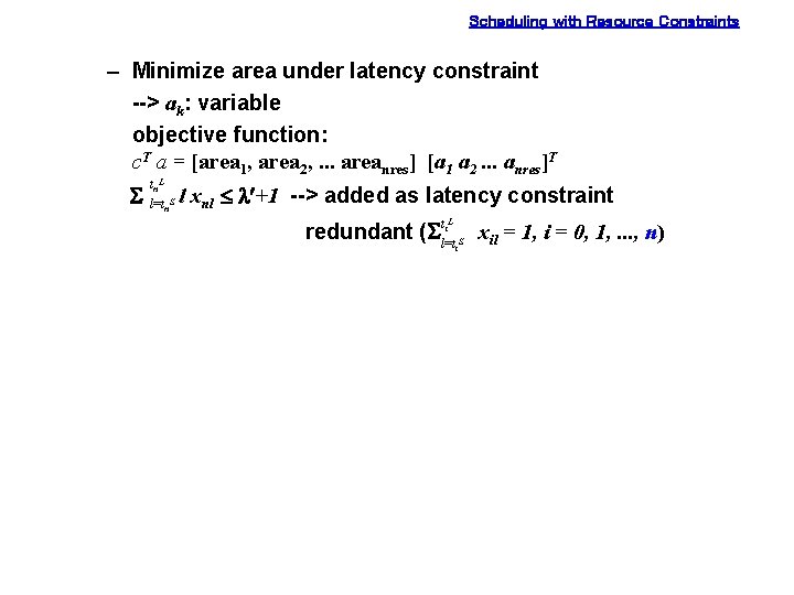
Scheduling with Resource Constraints – Minimize area under latency constraint --> ak: variable objective function: c. T a = [area 1, area 2, . . . areanres] [a 1 a 2. . . anres]T S tn. L l=tn. S l xnl £ l¢+1 --> added as latency constraint redundant (S ti. L l=ti. S xil = 1, i = 0, 1, . . . , n)

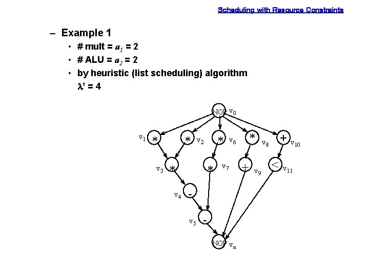
Scheduling with Resource Constraints – Example 1 • # mult = a 1 = 2 • # ALU = a 2 = 2 • by heuristic (list scheduling) algorithm l’ = 4 NOP v 0 v 1 * v 3 * * v 4 * v 2 * v 7 v 5 * v 6 NOP vn + v 9 + v 10 v 8 < v 11

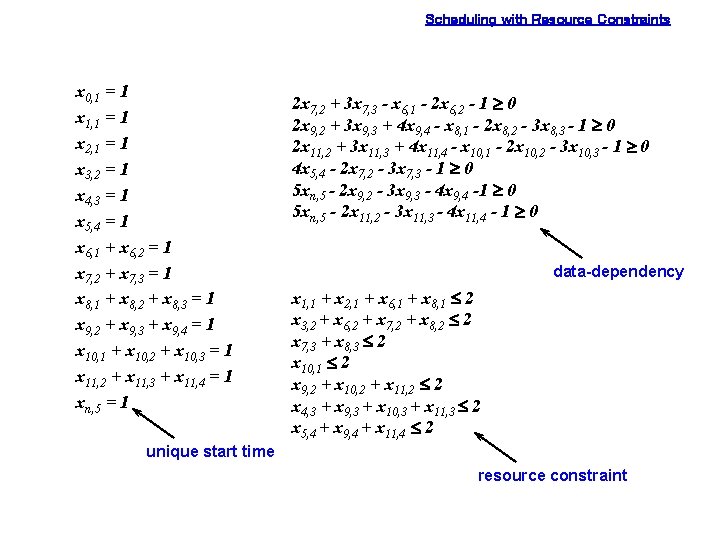
Scheduling with Resource Constraints x 0, 1 = 1 x 1, 1 = 1 x 2, 1 = 1 x 3, 2 = 1 x 4, 3 = 1 x 5, 4 = 1 x 6, 1 + x 6, 2 = 1 x 7, 2 + x 7, 3 = 1 x 8, 1 + x 8, 2 + x 8, 3 = 1 x 9, 2 + x 9, 3 + x 9, 4 = 1 x 10, 1 + x 10, 2 + x 10, 3 = 1 x 11, 2 + x 11, 3 + x 11, 4 = 1 xn, 5 = 1 2 x 7, 2 + 3 x 7, 3 - x 6, 1 - 2 x 6, 2 - 1 ³ 0 2 x 9, 2 + 3 x 9, 3 + 4 x 9, 4 - x 8, 1 - 2 x 8, 2 - 3 x 8, 3 - 1 ³ 0 2 x 11, 2 + 3 x 11, 3 + 4 x 11, 4 - x 10, 1 - 2 x 10, 2 - 3 x 10, 3 - 1 ³ 0 4 x 5, 4 - 2 x 7, 2 - 3 x 7, 3 - 1 ³ 0 5 xn, 5 - 2 x 9, 2 - 3 x 9, 3 - 4 x 9, 4 -1 ³ 0 5 xn, 5 - 2 x 11, 2 - 3 x 11, 3 - 4 x 11, 4 - 1 ³ 0 data-dependency x 1, 1 + x 2, 1 + x 6, 1 + x 8, 1 £ 2 x 3, 2 + x 6, 2 + x 7, 2 + x 8, 2 £ 2 x 7, 3 + x 8, 3 £ 2 x 10, 1 £ 2 x 9, 2 + x 10, 2 + x 11, 2 £ 2 x 4, 3 + x 9, 3 + x 10, 3 + x 11, 3 £ 2 x 5, 4 + x 9, 4 + x 11, 4 £ 2 unique start time resource constraint

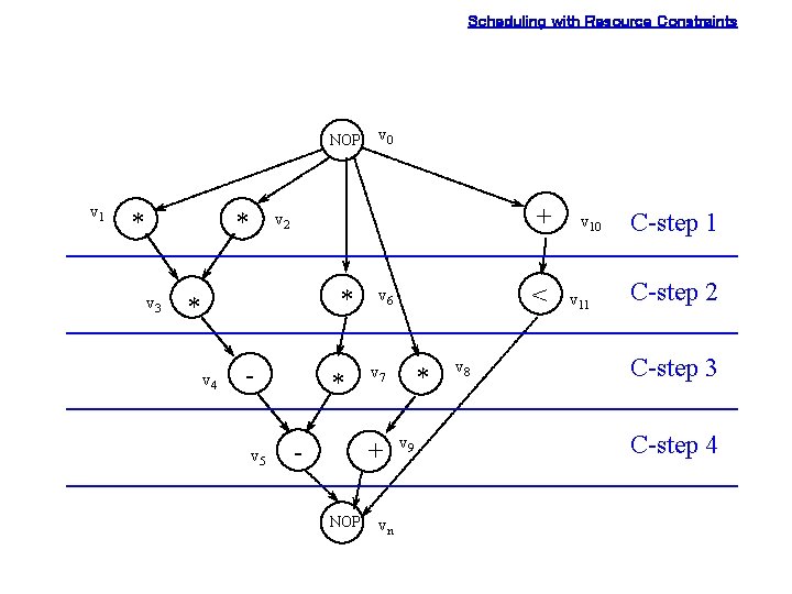
Scheduling with Resource Constraints NOP v 1 * * v 3 + v 2 * * v 4 v 0 v 5 * v 7 + NOP < v 6 vn * v 9 v 8 v 10 v 11 C-step 2 C-step 3 C-step 4

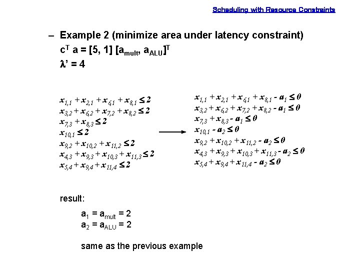
Scheduling with Resource Constraints – Example 2 (minimize area under latency constraint) c. T a = [5, 1] [amult, a. ALU]T l’ = 4 x 1, 1 + x 2, 1 + x 6, 1 + x 8, 1 £ 2 x 3, 2 + x 6, 2 + x 7, 2 + x 8, 2 £ 2 x 7, 3 + x 8, 3 £ 2 x 10, 1 £ 2 x 9, 2 + x 10, 2 + x 11, 2 £ 2 x 4, 3 + x 9, 3 + x 10, 3 + x 11, 3 £ 2 x 5, 4 + x 9, 4 + x 11, 4 £ 2 x 1, 1 + x 2, 1 + x 6, 1 + x 8, 1 - a 1 £ 0 x 3, 2 + x 6, 2 + x 7, 2 + x 8, 2 - a 1 £ 0 x 7, 3 + x 8, 3 - a 1 £ 0 x 10, 1 - a 2 £ 0 x 9, 2 + x 10, 2 + x 11, 2 - a 2 £ 0 x 4, 3 + x 9, 3 + x 10, 3 + x 11, 3 - a 2 £ 0 x 5, 4 + x 9, 4 + x 11, 4 - a 2 £ 0 result: a 1 = amult = 2 a 2 = a. ALU = 2 same as the previous example

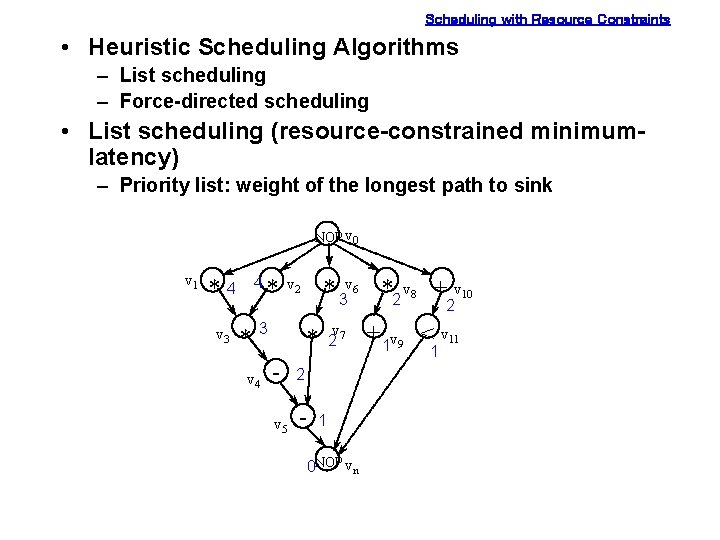
Scheduling with Resource Constraints • Heuristic Scheduling Algorithms – List scheduling – Force-directed scheduling • List scheduling (resource-constrained minimumlatency) – Priority list: weight of the longest path to sink NOP v 0 v 1 4 *4 v 3 * * 2 3 v 4 * 3 v 6 *2 v 8 + v 10 v 2 * - 2 v 5 - v 27 1 0 NOP vn + 1 v 9 < v 11 1

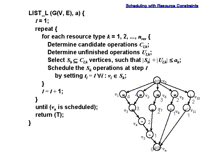
Scheduling with Resource Constraints LIST_L (G(V, E), a) { l = 1; repeat { for each resource type k = 1, 2, . . . , nres { Determine candidate operations Cl, k; Determine unfinished operations Ul, k; Select Sk Í Cl, k vertices, such that |Sk| + |Ul, k| £ ak; Schedule the Sk operations at step l by setting ti = l "i : vi Î Sk; NOP v 0 } l = l + 1; v 1 4 4 * v 2 * v 6 * v 8 + v 10 * } 3 2 2 until (vn is scheduled); v v 3 * 3 2 7 + 1 v 9 < v 11 * return (T); 1 } v 4 - 2 v 5 - 1 0 NOP vn

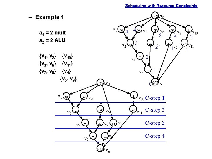
Scheduling with Resource Constraints NOP v 0 – Example 1 v 1 a 1 = 2 mult a 2 = 2 ALU {v 1, v 2} {v 3, v 6} {v 7, v 8} v 3 {v 10} {v 11} {v 4} {v 5, v 9} v 1 * v 3 * NOP v 0 v 5 + - * v 6 * v 7 2 * - 2 v 5 - + 1 v 9 < v 11 v 27 1 1 v 10 C-step 1 < v 11 C-step 2 * + v 9 NOP vn * 3 v 6 *2 v 8 + v 10 v 2 0 NOP vn v 2 * * 3 v 4 * v 4 4 *4 v 8 C-step 3 C-step 4

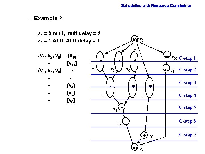
Scheduling with Resource Constraints – Example 2 a 1 = 3 mult, mult delay = 2 a 2 = 1 ALU, ALU delay = 1 {v 1, v 2, v 6} {v 3, v 7, v 8} - {v 10} {v 11} {v 4} {v 5} {v 9} NOP v 0 * v 1 * v 2 * v 6 * * v 3 v 7 v 4 * v 8 v 10 C-step 1 < v 11 C-step 2 C-step 3 C-step 4 v 5 + C-step 5 - C-step 6 + NOP vn v 9 C-step 7

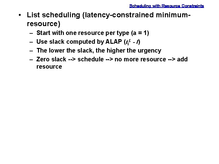
Scheduling with Resource Constraints • List scheduling (latency-constrained minimumresource) – – Start with one resource per type (a = 1) Use slack computed by ALAP (ti. L - l) The lower the slack, the higher the urgency Zero slack --> schedule --> no more resource --> add resource

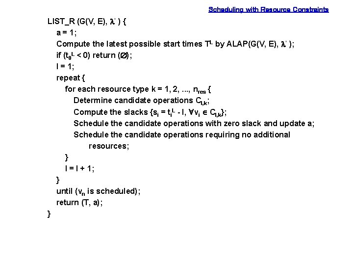
Scheduling with Resource Constraints LIST_R (G(V, E), l’ ) { a = 1; Compute the latest possible start times TL by ALAP(G(V, E), l’ ); if (t 0 L < 0) return (Æ); l = 1; repeat { for each resource type k = 1, 2, . . . , nres { Determine candidate operations Cl, k; Compute the slacks {si = ti. L - l, "vi Î Cl, k}; Schedule the candidate operations with zero slack and update a; Schedule the candidate operations requiring no additional resources; } l = l + 1; } until (vn is scheduled); return (T, a); }

Scheduling with Resource Constraints • Example zero slack a = [1, 1]T {v 1, v 2} ---> a = [2, 1]T {v 3, v 6} {v 7, v 8} {v 10} {v 11} {v 4} {v 5, v 9} ---> a = [2, 2]T NOP v 0 v 1 * v 3 * * * v 4 + v 2 v 5 * < v 6 * v 7 - + NOP vn v 9 v 11 + v 8 < v 10 C-step v 10 v 11 1 C-step 2 C-step 3 C-step 4

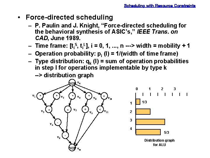
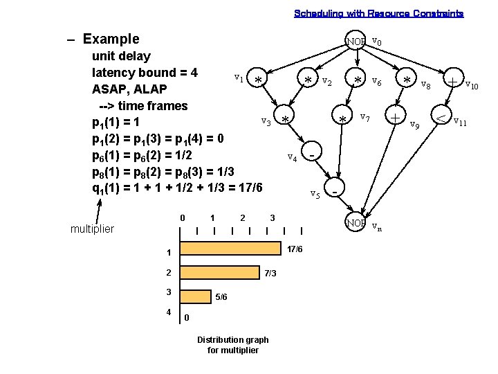
Scheduling with Resource Constraints • Force-directed scheduling – P. Paulin and J. Knight, “Force-directed scheduling for the behavioral synthesis of ASIC’s, ” IEEE Trans. on CAD, June 1989. – Time frame: [ti. S, ti. L], i = 0, 1, . . . , n ---> width = mobility + 1 – Operation probability: pi (l) = 1/(width of time frame) – Type distribution: qk (l) = sum of operation probabilities in step l for operations implementable by type k --> distribution graph NOP v 0 0 v 1 * * * v 2 * v 6 v 8 + v 10 1 v 3 * * v 4 v 7 + v 9 < v 11 2 3 1/3 2 3 - 4 v 5 1 - NOP vn 5/3 Distribution graph for ALU

Scheduling with Resource Constraints – Example NOP v 0 unit delay latency bound = 4 v 1 * ASAP, ALAP --> time frames v 3 p 1(1) = 1 p 1(2) = p 1(3) = p 1(4) = 0 p 6(1) = p 6(2) = 1/2 p 8(1) = p 8(2) = p 8(3) = 1/3 q 1(1) = 1 + 1/2 + 1/3 = 17/6 0 multiplier 1 2 * * v 4 3 7/3 4 5/6 0 Distribution graph for multiplier * v 6 v 7 NOP vn 17/6 3 * v 5 1 2 * v 2 + v 9 + v 8 < v 10 v 11

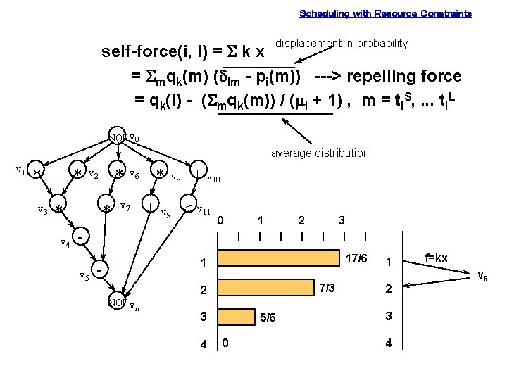
Scheduling with Resource Constraints displacement in probability self-force(i, l) = S k x = Smqk(m) (dlm - pi(m)) ---> repelling force = qk(l) - (Smqk(m)) / (mi + 1) , m = ti. S, . . . ti. L NOP v 0 average distribution v 1 * v 3 * * v 4 * v 2 * * v 6 v 7 + v 8 v 9 + v 10 < v 11 0 1 2 3 v 5 17/6 1 - 7/3 2 NOP vn 3 4 5/6 0 1 2 3 4 f=kx v 6

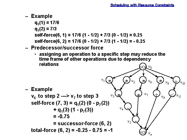
Scheduling with Resource Constraints – Example q 1(1) = 17/6 q 1(2) = 7/3 self-force(6, 1) = 17/6 (1 - 1/2) + 7/3 (0 - 1/2) = 0. 25 self-force(6, 2) = 17/6 (0 - 1/2) + 7/3 (1 - 1/2) = - 0. 25 – Predecessor/successor force • assigning an operation to a specific step may reduce the time frame of other operations due to dependency relations v NOP v 1 * * v 2 * 0 v 6 – Example v 3 * v 6 to step 2 ---> v 7 to step 3 * v 7 + self-force (7, 3) = q 1(2) (0 - p 7(2)) v 4 + q 1(3) (1 - p 7(3)) = -0. 75 v 5 = successor-force (6, 2) total-force (6, 2) = -0. 25 - 0. 75 = -1 NOP v n * v 9 + v 8 < v 10 v 11

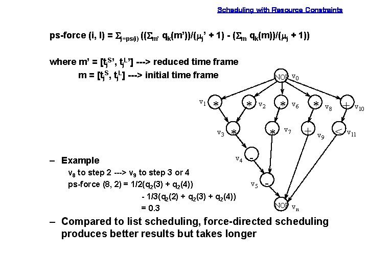
Scheduling with Resource Constraints ps-force (i, l) = Sj=ps(i) ((Sm’ qk(m’))/(mj’ + 1) - (Sm qk(m))/(mj + 1)) where m’ = [tj. S’, tj. L’] ---> reduced time frame m = [tj. S, tj. L] ---> initial time frame v 1 * v 3 – Example NOP v 0 * * v 4 v 8 to step 2 ---> v 9 to step 3 or 4 ps-force (8, 2) = 1/2(q 2(3) + q 2(4)) - 1/3(q 2(2) + q 2(3) + q 2(4)) = 0. 3 * v 2 * * v 6 v 7 + v 9 v 5 + v 8 NOP vn – Compared to list scheduling, force-directed scheduling produces better results but takes longer < v 10 v 11

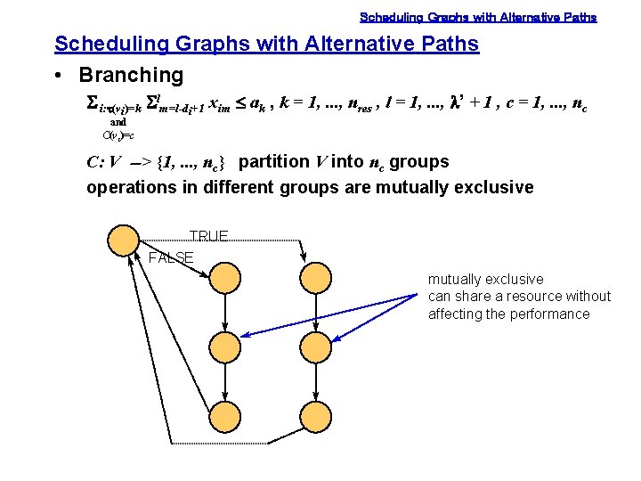
Scheduling Graphs with Alternative Paths • Branching S i: t(vi)=k Slm=l-di+1 xim £ ak , k = 1, . . . , nres , l = 1, . . . , l’ + 1 , c = 1, . . . , nc and C(vi)=c C: V --> {1, . . . , nc} partition V into nc groups operations in different groups are mutually exclusive TRUE FALSE mutually exclusive can share a resource without affecting the performance

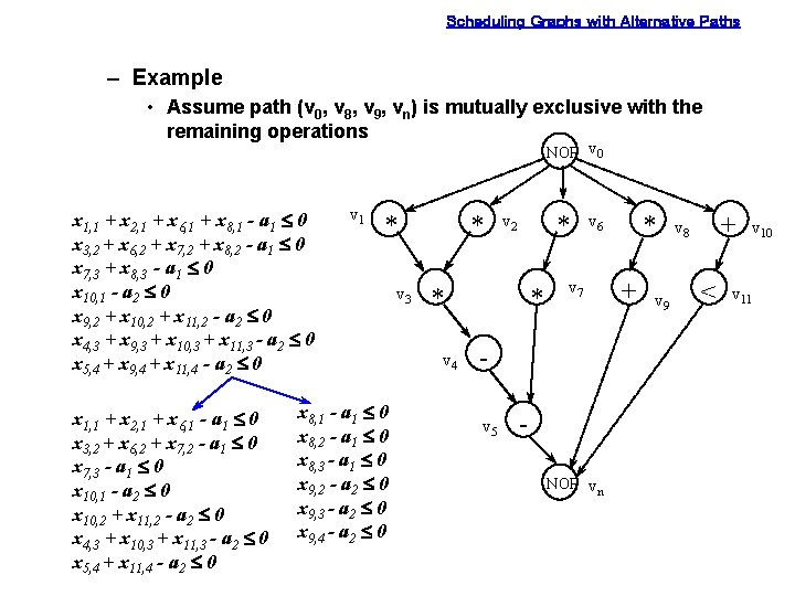
Scheduling Graphs with Alternative Paths – Example • Assume path (v 0, v 8, v 9, vn) is mutually exclusive with the remaining operations NOP v 0 x 1, 1 + x 2, 1 + x 6, 1 + x 8, 1 - a 1 £ 0 x 3, 2 + x 6, 2 + x 7, 2 + x 8, 2 - a 1 £ 0 x 7, 3 + x 8, 3 - a 1 £ 0 x 10, 1 - a 2 £ 0 x 9, 2 + x 10, 2 + x 11, 2 - a 2 £ 0 x 4, 3 + x 9, 3 + x 10, 3 + x 11, 3 - a 2 £ 0 x 5, 4 + x 9, 4 + x 11, 4 - a 2 £ 0 x 1, 1 + x 2, 1 + x 6, 1 - a 1 £ 0 x 3, 2 + x 6, 2 + x 7, 2 - a 1 £ 0 x 7, 3 - a 1 £ 0 x 10, 1 - a 2 £ 0 x 10, 2 + x 11, 2 - a 2 £ 0 x 4, 3 + x 10, 3 + x 11, 3 - a 2 £ 0 x 5, 4 + x 11, 4 - a 2 £ 0 v 1 * x 8, 1 - a 1 £ 0 x 8, 2 - a 1 £ 0 x 8, 3 - a 1 £ 0 x 9, 2 - a 2 £ 0 x 9, 3 - a 2 £ 0 x 9, 4 - a 2 £ 0 v 3 * * v 2 * v 4 * v 7 v 5 * v 6 NOP vn + v 9 + v 8 < v 10 v 11

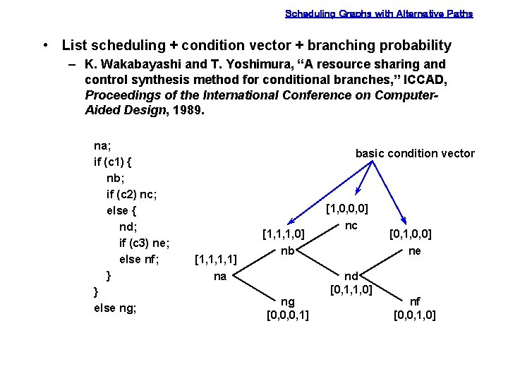
Scheduling Graphs with Alternative Paths • List scheduling + condition vector + branching probability – K. Wakabayashi and T. Yoshimura, “A resource sharing and control synthesis method for conditional branches, ” ICCAD, Proceedings of the International Conference on Computer. Aided Design, 1989. na; if (c 1) { nb; if (c 2) nc; else { nd; if (c 3) ne; else nf; } } else ng; basic condition vector [1, 1, 1, 1] na [1, 1, 1, 0] nb ng [0, 0, 0, 1] [1, 0, 0, 0] nc nd [0, 1, 1, 0] [0, 1, 0, 0] ne nf [0, 0, 1, 0]

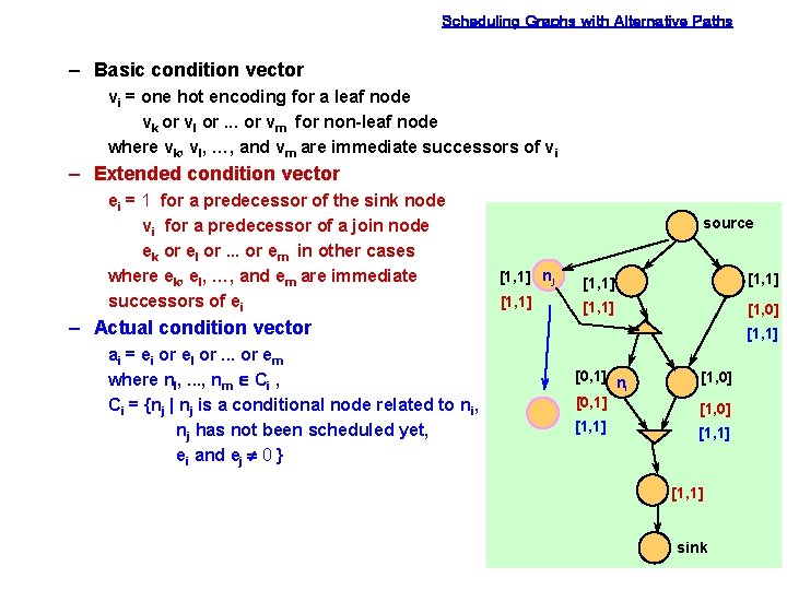
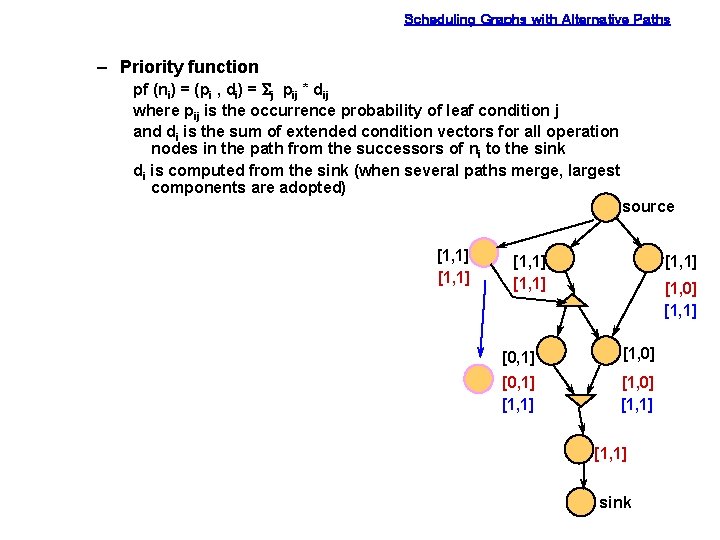
Scheduling Graphs with Alternative Paths – Basic condition vector vi = one hot encoding for a leaf node vk or vl or. . . or vm for non-leaf node where vk, vl, …, and vm are immediate successors of vi – Extended condition vector ei = 1 for a predecessor of the sink node vi for a predecessor of a join node ek or el or. . . or em in other cases where ek, el, …, and em are immediate successors of ei source [1, 1] nj [1, 1] [1, 0] – Actual condition vector ai = ei or el or. . . or em where nl, . . . , nm Î Ci , Ci = {nj | nj is a conditional node related to ni, nj has not been scheduled yet, ei and ej ¹ 0 } [1, 1] [0, 1] n i [0, 1] [1, 0] [1, 1] sink

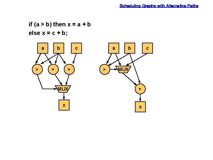
Scheduling Graphs with Alternative Paths if (a > b) then x = a + b else x = c + b; a > b c + + a > b c MUX + x x

Scheduling Graphs with Alternative Paths – Priority function pf (ni) = (pi , di) = Sj pij * dij where pij is the occurrence probability of leaf condition j and di is the sum of extended condition vectors for all operation nodes in the path from the successors of ni to the sink di is computed from the sink (when several paths merge, largest components are adopted) source [1, 1] [1, 1] [1, 0] [1, 1] [0, 1] [1, 0] [1, 1] sink

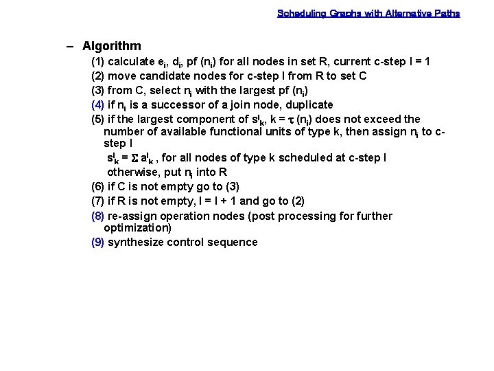
Scheduling Graphs with Alternative Paths – Algorithm (1) calculate ei, di, pf (ni) for all nodes in set R, current c-step l = 1 (2) move candidate nodes for c-step l from R to set C (3) from C, select ni with the largest pf (ni) (4) if ni is a successor of a join node, duplicate (5) if the largest component of slk, k = t (ni) does not exceed the number of available functional units of type k, then assign ni to cstep l slk = S alk , for all nodes of type k scheduled at c-step l otherwise, put ni into R (6) if C is not empty go to (3) (7) if R is not empty, l = l + 1 and go to (2) (8) re-assign operation nodes (post processing for further optimization) (9) synthesize control sequence

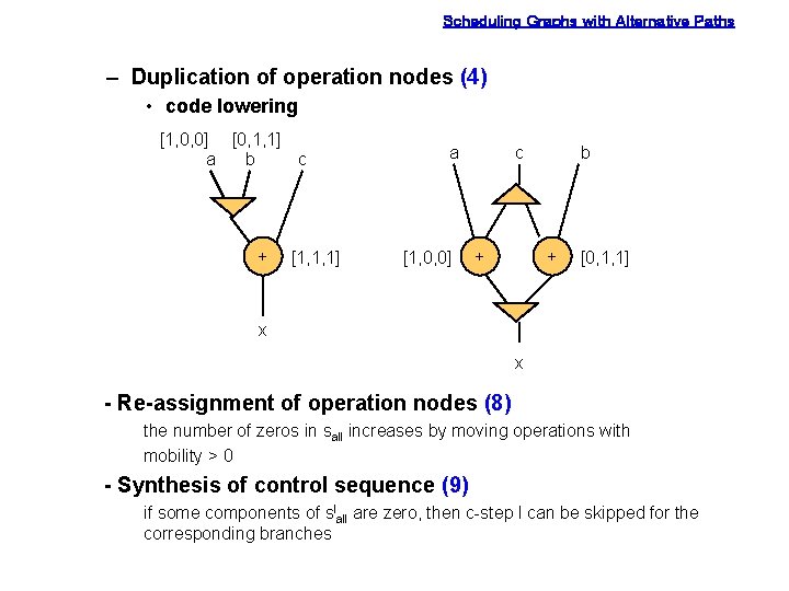
Scheduling Graphs with Alternative Paths – Duplication of operation nodes (4) • code lowering [1, 0, 0] [0, 1, 1] a b c + [1, 1, 1] a [1, 0, 0] c + b + [0, 1, 1] x x - Re-assignment of operation nodes (8) the number of zeros in sall increases by moving operations with mobility > 0 - Synthesis of control sequence (9) if some components of slall are zero, then c-step l can be skipped for the corresponding branches

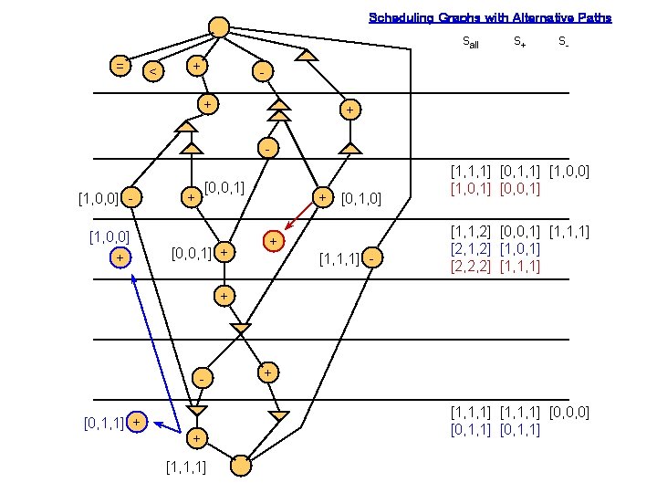
Scheduling Graphs with Alternative Paths sall = < + s+ s- + + - [1, 0, 0] + [0, 0, 1] + + [0, 1, 0] + [1, 1, 1] - [1, 1, 1] [0, 1, 1] [1, 0, 0] [1, 0, 1] [0, 0, 1] [1, 1, 2] [0, 0, 1] [1, 1, 1] [2, 1, 2] [1, 0, 1] [2, 2, 2] [1, 1, 1] + [0, 1, 1] + + [1, 1, 1] [0, 0, 0] [0, 1, 1]

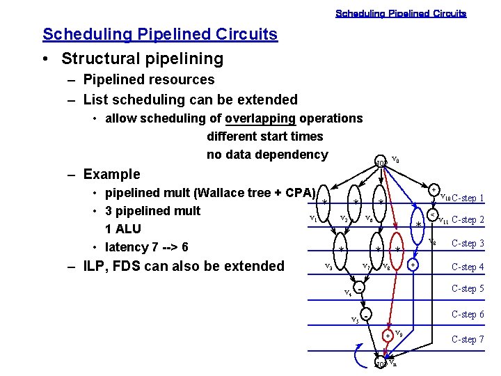
Scheduling Pipelined Circuits • Structural pipelining – Pipelined resources – List scheduling can be extended • allow scheduling of overlapping operations different start times no data dependency NOP – Example • pipelined mult (Wallace tree + CPA) * * • 3 pipelined mult v 1 v 2 1 ALU • latency 7 --> 6 * – ILP, FDS can also be extended v 3 + * v 6 * * v 7 v 4 v 0 * + v 8 - v 5 v 10 C-step 1 < v 11 C-step 2 v 8 C-step 3 C-step 4 C-step 5 - C-step 6 + v 9 NOP vn C-step 7

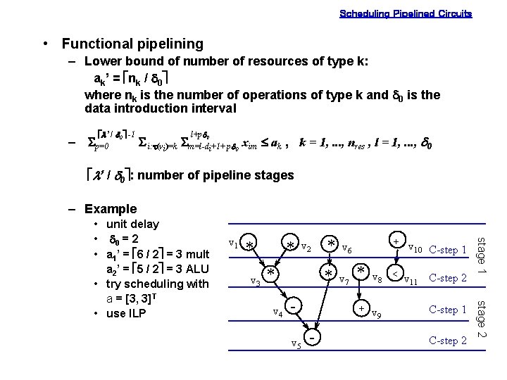
Scheduling Pipelined Circuits • Functional pipelining – Lower bound of number of resources of type k: ak’ = énk / d 0ù where nk is the number of operations of type k and d 0 is the data introduction interval él’ / d 0ù -1 – Sp=0 l+pd 0 S i: t(vi)=k Sm=l-di+1+ pd 0 xim £ ak , k = 1, . . . , nres , l = 1, . . . , d 0 él’ / d 0ù: number of pipeline stages – Example v 1 * v 3 * v 2 * v 5 v 6 * v 7 + * v 8 < v 11 + v 9 - v 10 C-step 1 C-step 2 stage 2 v 4 * stage 1 • unit delay • d 0 = 2 • a 1’ = é 6 / 2ù = 3 mult a 2’ = é 5 / 2ù = 3 ALU • try scheduling with a = [3, 3]T • use ILP

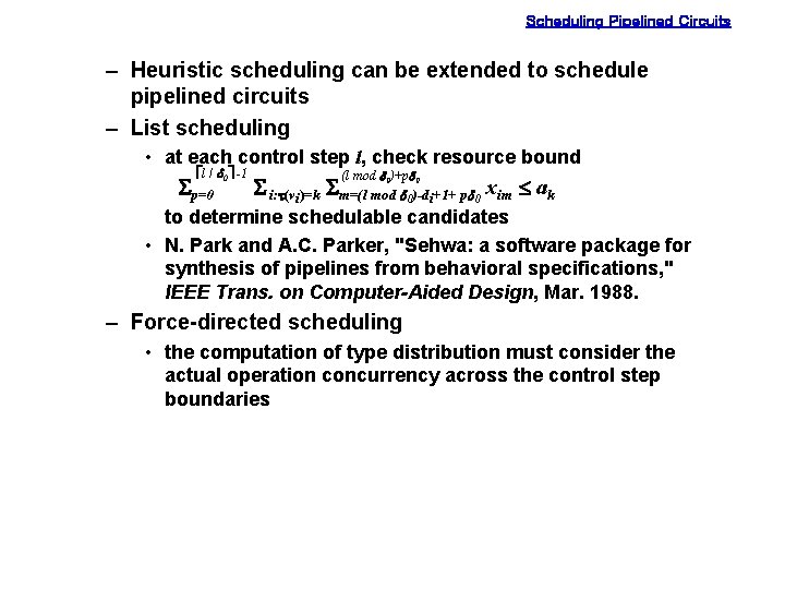
Scheduling Pipelined Circuits – Heuristic scheduling can be extended to schedule pipelined circuits – List scheduling • at each control step l, check resource bound él / d 0ù -1 Sp=0 (l mod d 0)+pd 0 S i: t(vi)=k Sm=(l mod d 0)-di+1+ pd 0 xim £ ak to determine schedulable candidates • N. Park and A. C. Parker, "Sehwa: a software package for synthesis of pipelines from behavioral specifications, " IEEE Trans. on Computer-Aided Design, Mar. 1988. – Force-directed scheduling • the computation of type distribution must consider the actual operation concurrency across the control step boundaries

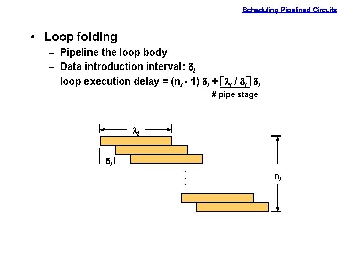
Scheduling Pipelined Circuits • Loop folding – Pipeline the loop body – Data introduction interval: dl loop execution delay = (nl - 1) dl + éll / dlù dl # pipe stage ll dl. . . nl

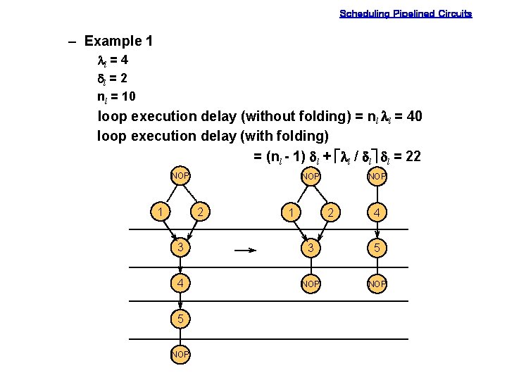
Scheduling Pipelined Circuits – Example 1 ll = 4 dl = 2 nl = 10 loop execution delay (without folding) = nl ll = 40 loop execution delay (with folding) = (nl - 1) dl + éll / dlù dl = 22 NOP 1 NOP 2 4 3 3 5 4 NOP 5 NOP

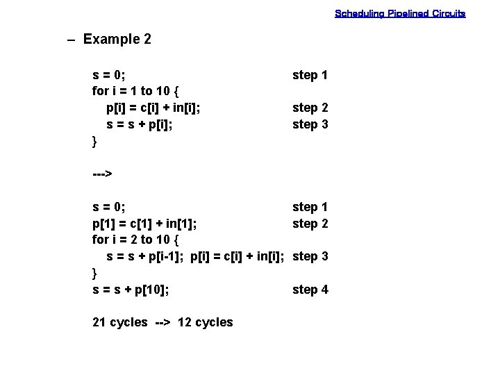
Scheduling Pipelined Circuits – Example 2 s = 0; for i = 1 to 10 { p[i] = c[i] + in[i]; s = s + p[i]; } step 1 step 2 step 3 ---> s = 0; p[1] = c[1] + in[1]; for i = 2 to 10 { s = s + p[i-1]; p[i] = c[i] + in[i]; } s = s + p[10]; 21 cycles --> 12 cycles step 1 step 2 step 3 step 4