Schaefer model through the Fish Banks role playing

Schaefer model through the Fish. Banks role playing game
Fish. Banks • Fish Banks – is a computer-assisted interactive, role-playing simulation in which groups manage a fishing company – Participants try to maximize their assets in a world with renewable natural resources and economic competition. – the game has been created in 1986 by Dennis Meadows • • A diversity of strategies Management of incomes or resources ? Free Access => negociations Discussion about the type of measurements – => need of an agreement about the diagnostic • Discussion <=> institution – Rules - Control - Sanctions 2 Espaces et Ressources
Fish. Banks A message Privatization of the profits, socialization of losses Social cost extern to the market A standard model Schaefer 3 Espaces et Ressources
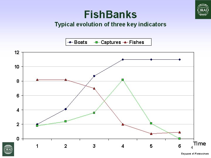
Fish. Banks Typical evolution of three key indicators Boats Captures Fishes 12 10 8 6 4 2 0 1 2 3 4 5 6 4 Time Espaces et Ressources

The Schaeffer model Carrying capacity K and equilibrium • Based on Verhulst model (Logistic equation) : dx/dt = rx (1 - x/K) + K/2 K x 5 Espaces et Ressources

Renewable resource with harvest h(t) • Constant harvest h(t) • dx/dt = rx (1 - x/K) - h(t) • MSH = Maximum sustainable harvest, XK/2 h. RMS + h - K X 1 =unstable equilibrium x X 2 =stable equilibrium 6 Espaces et Ressources

Harvest h(t) with effort E and capturability q • Harvest: h(t) = q. E. x • Fishing effort E (number of boats), q capturability • dx/dt = rx (1 - x/K) - h(t) + . x E. q h + -- h’ x q. E’. K X =Equilibrium =Equilibre x 7 Espaces et Ressources

Renewable resource Harvest h(t) with effort E and capturability q • dx/dt = rx (1 - x/K) - h(t) • h(t) = q. E. x At the biological equilibrium, one harvests what is produced . x E. q x* 8 Espaces et Ressources
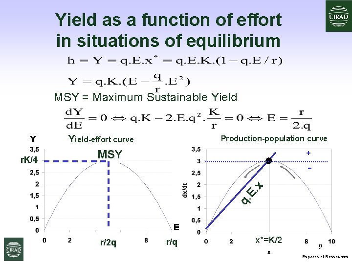
Yield as a function of effort in situations of equilibrium MSY = Maximum Sustainable Yield Production-population curve MSY + x r. K/4 Yield-effort curve q. E. Y E r/2 q r/q x*=K/2 9 Espaces et Ressources

Renewable resource Estimation of the parameters • h=Y = q. E. x* = q. E. K. (1 - q. E/r) • Y/E = -(q 2. K/r). E +q. K Catches per ship Y/E Capture per effort – effort curve The Schaefer line q. K Y/EMSY=q. K/2 -q 2. K/ r EMSY=r/2 q r/q E Number of ships 10 Espaces et Ressources
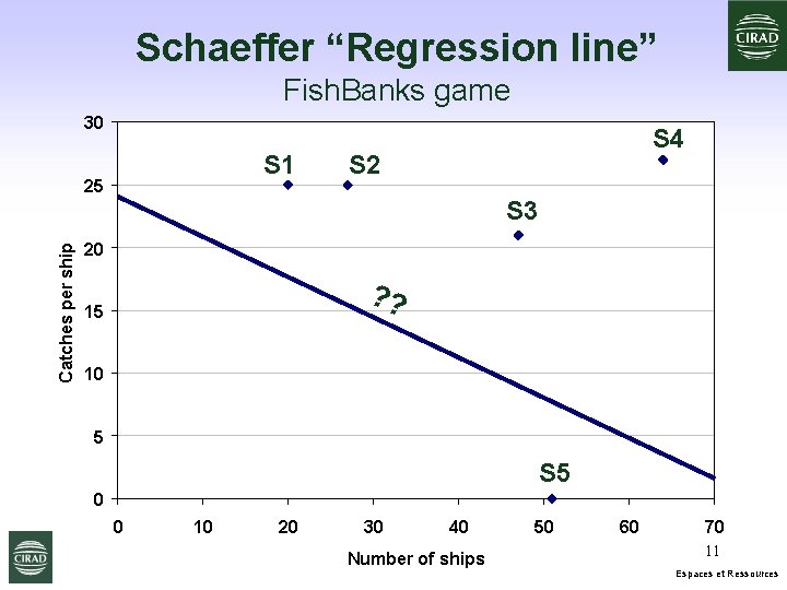
Schaeffer “Regression line” Fish. Banks game 30 S 1 Catches per ship 25 S 4 S 2 S 3 20 ? ? 15 10 5 S 5 0 0 10 20 30 40 Number of ships 50 60 70 11 Espaces et Ressources
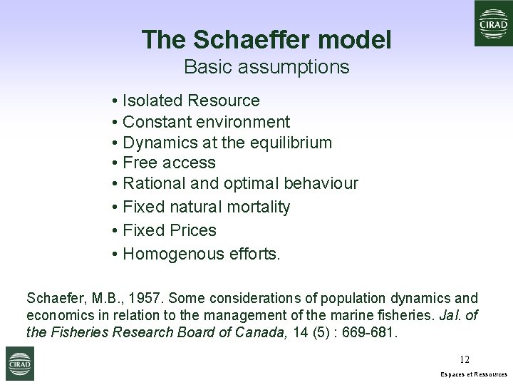
The Schaeffer model Basic assumptions • Isolated Resource • Constant environment • Dynamics at the equilibrium • Free access • Rational and optimal behaviour • Fixed natural mortality • Fixed Prices • Homogenous efforts. Schaefer, M. B. , 1957. Some considerations of population dynamics and economics in relation to the management of the marine fisheries. Jal. of the Fisheries Research Board of Canada, 14 (5) : 669 -681. 12 Espaces et Ressources
Discrete Systems Dynamics Espaces et Ressources

Definitions • The state of the system at time t Xt = (at, bt, …) • The state at time t+1 only depends on the state at time t Xt+1= F(Xt) • X 0 and the function F are sufficient to define all possible values No need to run simulation to solve the system 14 Espaces et Ressources
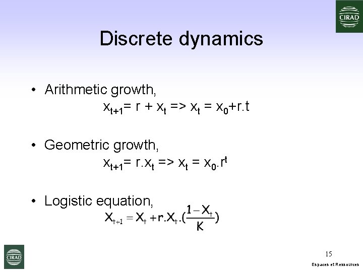
Discrete dynamics • Arithmetic growth, xt+1= r + xt => xt = x 0+r. t • Geometric growth, xt+1= r. xt => xt = x 0. rt • Logistic equation, 15 Espaces et Ressources

Linear equation Xt+1 = f(Xt) Xt = g(Xo, t) 16 Espaces et Ressources
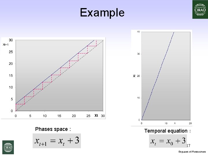
Example Phases space : Temporal equation : 17 Espaces et Ressources
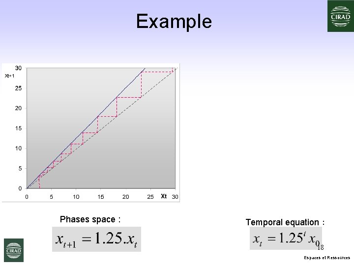
Example Phases space : Temporal equation : 18 Espaces et Ressources
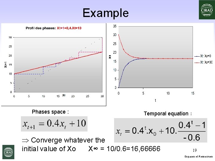
Example Phases space : Temporal equation : Þ Converge whatever the initial value of Xo X∞ = 10/0. 6=16, 66666 19 Espaces et Ressources
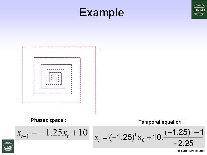
Example Phases space : Temporal equation : 20 Espaces et Ressources
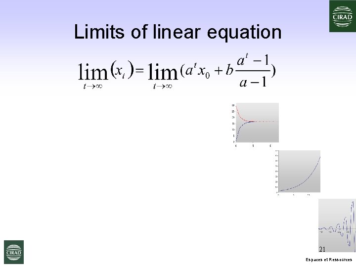
Limits of linear equation 21 Espaces et Ressources
Attractors • An attractor is a point or a set of points • Fixed point xt+1=xt • Cyclic point xt+n=xt 22 Espaces et Ressources
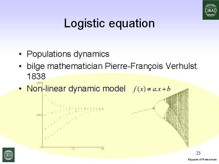
Logistic equation • Populations dynamics • bilge mathematician Pierre-François Verhulst. 1838 • Non-linear dynamic model 23 Espaces et Ressources
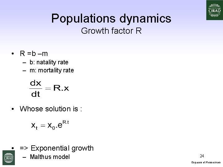
Populations dynamics Growth factor R • R =b –m – b: natality rate – m: mortality rate • Whose solution is : • => Exponential growth – Malthus model 24 Espaces et Ressources
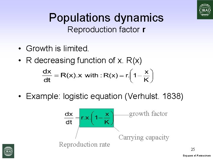
Populations dynamics Reproduction factor r • Growth is limited. • R decreasing function of x. R(x) • Example: logistic equation (Verhulst. 1838) growth factor Reproduction rate Carrying capacity 25 Espaces et Ressources
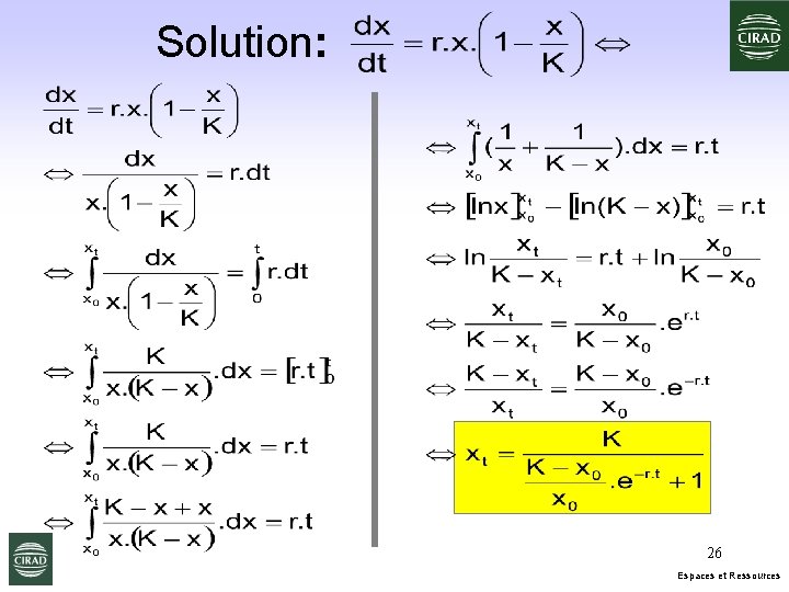
Solution: 26 Espaces et Ressources
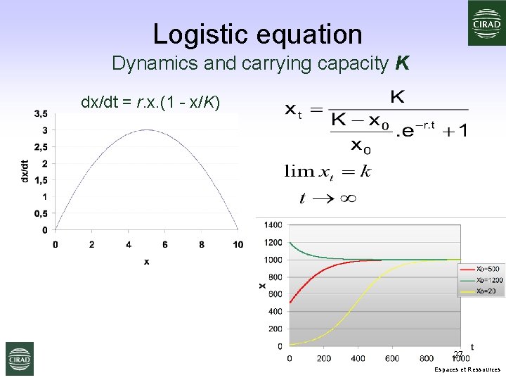
Logistic equation Dynamics and carrying capacity K dx/dt = r. x. (1 - x/K) 27 Espaces et Ressources
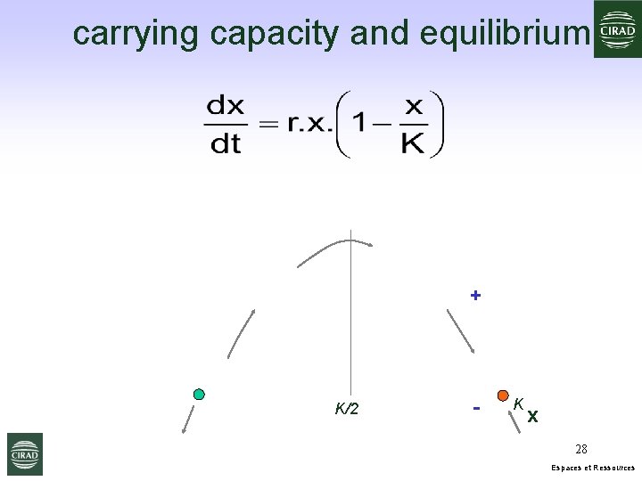
carrying capacity and equilibrium + K/2 - K x 28 Espaces et Ressources
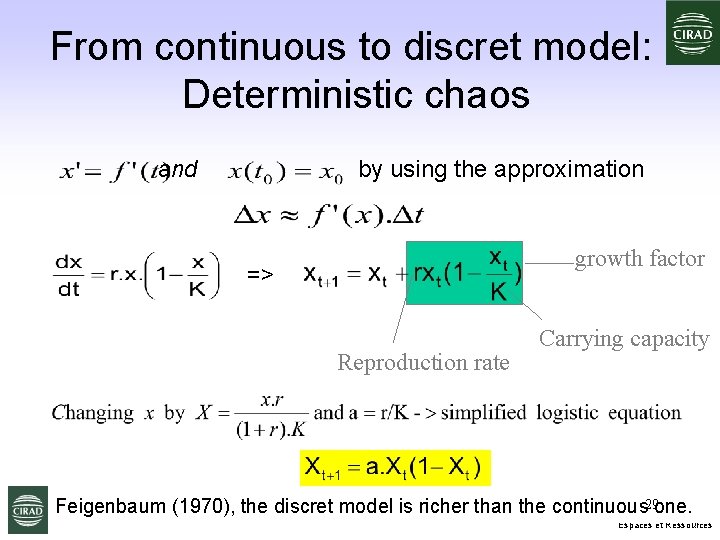
From continuous to discret model: Deterministic chaos and by using the approximation growth factor => Reproduction rate Carrying capacity Feigenbaum (1970), the discret model is richer than the continuous 29 one. Espaces et Ressources
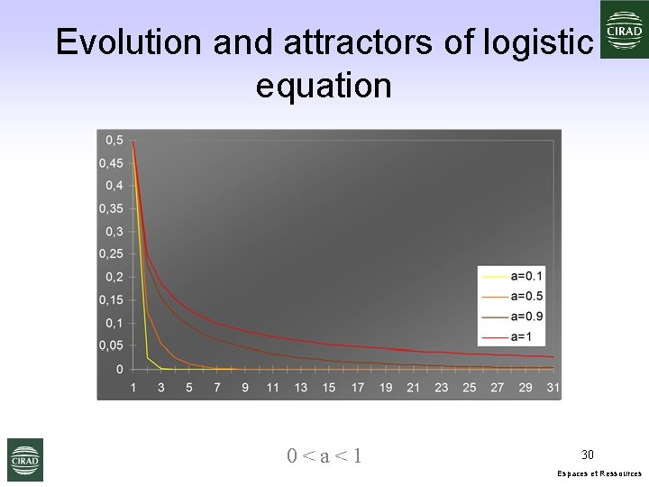
Evolution and attractors of logistic equation 0<a<1 30 Espaces et Ressources
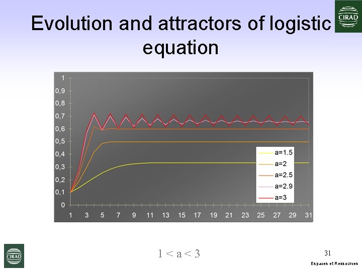
Evolution and attractors of logistic equation 1<a<3 31 Espaces et Ressources
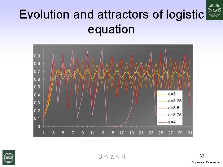
Evolution and attractors of logistic equation 3<a<4 32 Espaces et Ressources
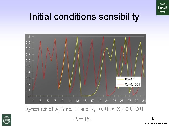
Initial conditions sensibility Dynamics of Xt for a =4 and X 0=0. 01 or X 0=0. 01001 Δ = 1‰ 33 Espaces et Ressources
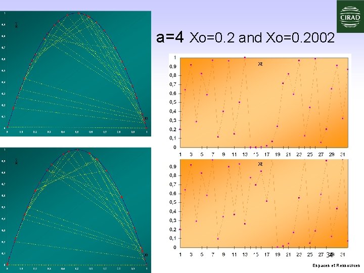
a=4 Xo=0. 2 and Xo=0. 2002 34 Espaces et Ressources
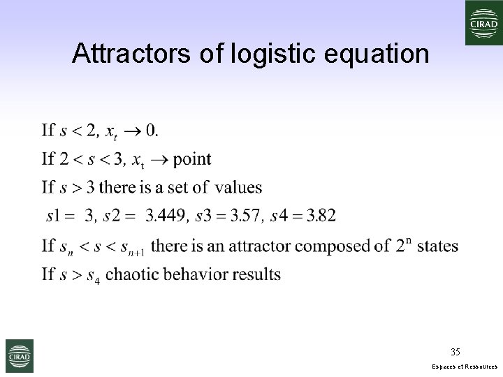
Attractors of logistic equation 35 Espaces et Ressources
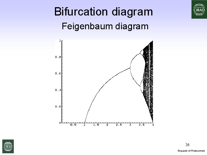
Bifurcation diagram Feigenbaum diagram 36 Espaces et Ressources
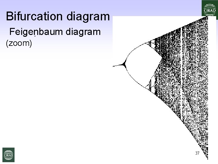
Bifurcation diagram Feigenbaum diagram (zoom) 37 Espaces et Ressources
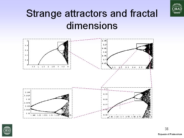
Strange attractors and fractal dimensions 38 Espaces et Ressources
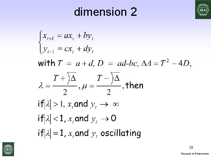
dimension 2 39 Espaces et Ressources

Henon attractor Attractor : shape You can’t predict x, y at t The system is organized fractal properties 40 Espaces et Ressources
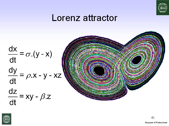
Lorenz attractor 41 Espaces et Ressources
References • Discrete system dynamics : Pavé, Tu, • Deterministic chaos : Casti, Cvitanovic • Discrete control : Clark 42 Espaces et Ressources
- Slides: 42