Scene planes and homographies Homographies given the plane

Scene planes and homographies

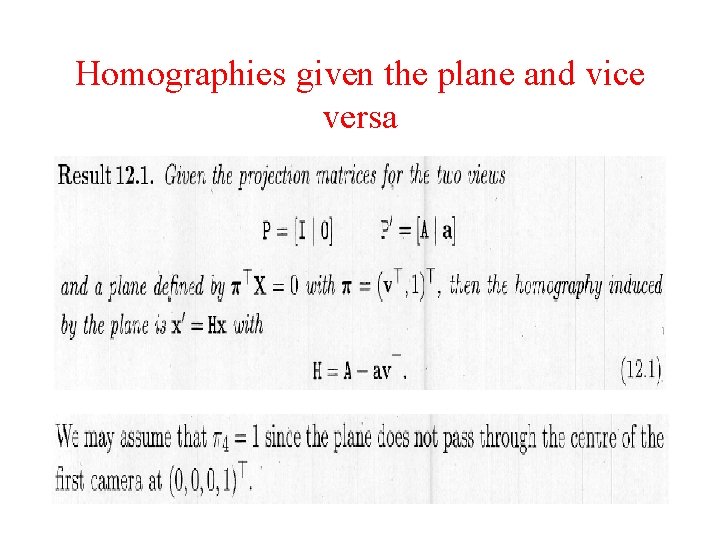
Homographies given the plane and vice versa

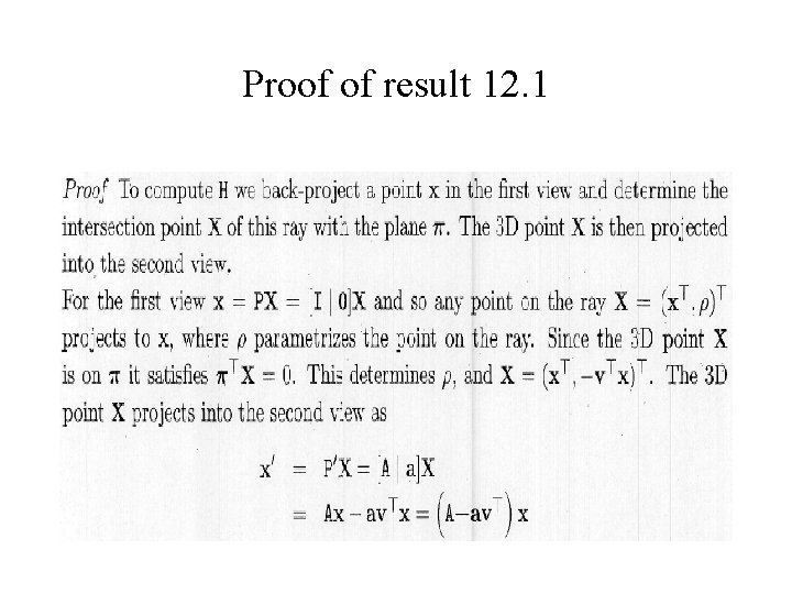
Proof of result 12. 1

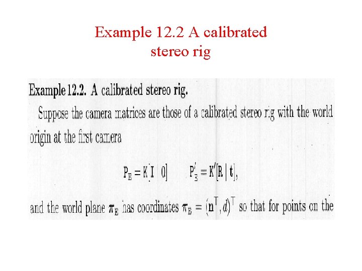
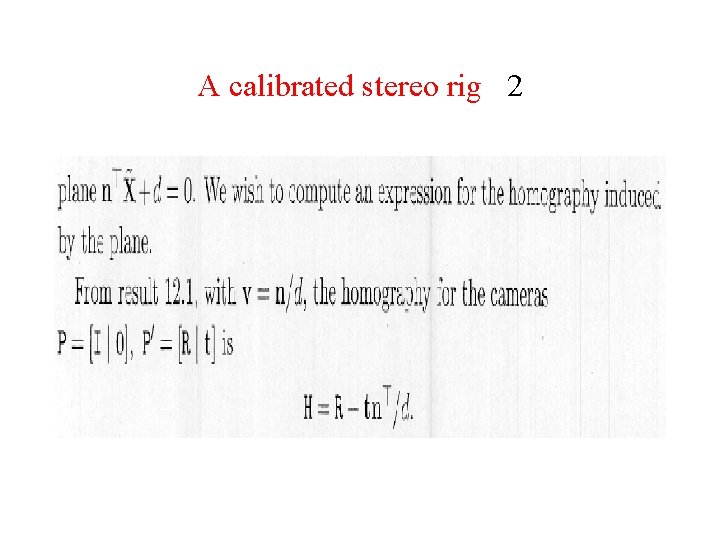
Example 12. 2 A calibrated stereo rig

A calibrated stereo rig 2

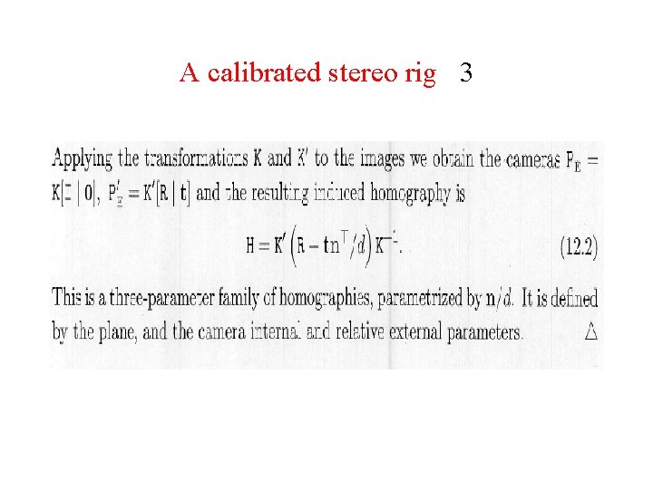
A calibrated stereo rig 3

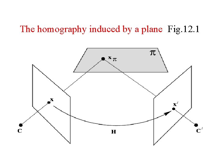
The homography induced by a plane Fig. 12. 1

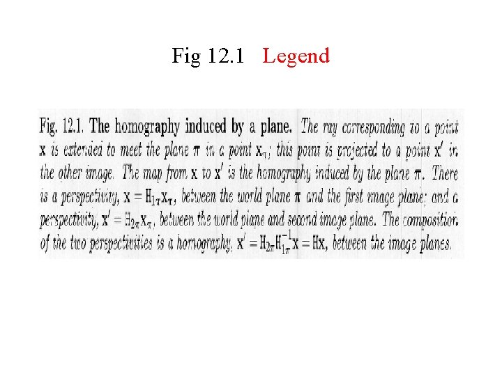
Fig 12. 1 Legend

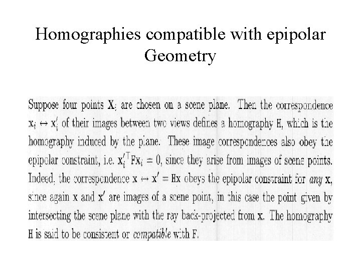
Homographies compatible with epipolar Geometry

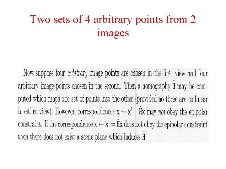
Two sets of 4 arbitrary points from 2 images

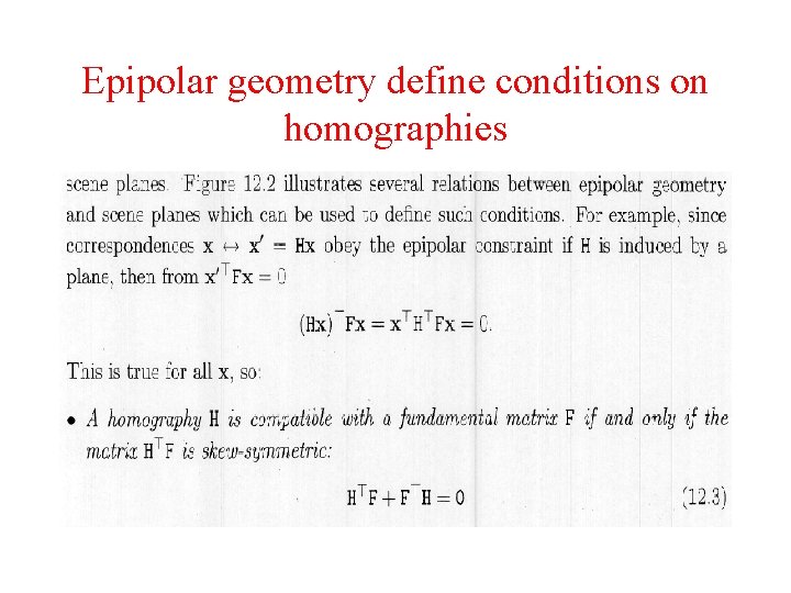
Epipolar geometry define conditions on homographies

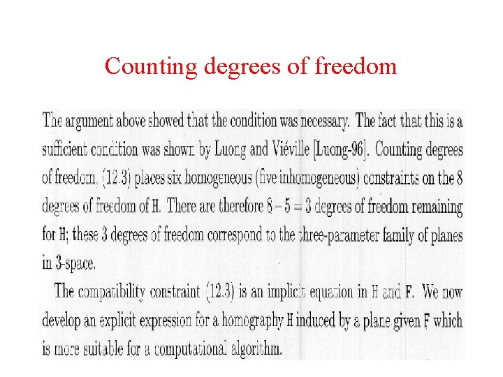
Counting degrees of freedom

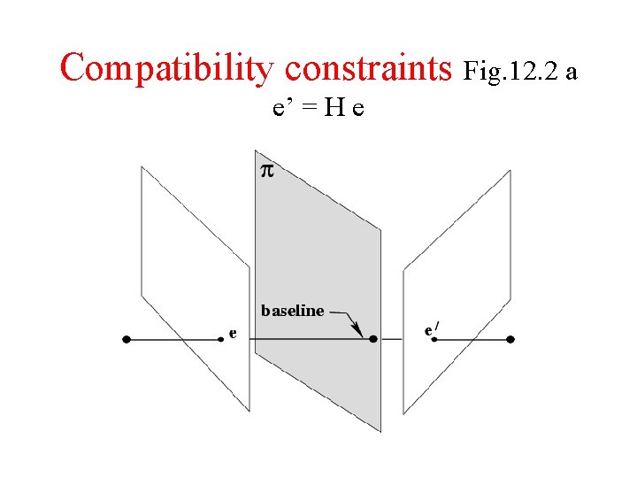
Compatibility constraints Fig. 12. 2 a e’ = H e

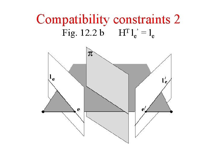
Compatibility constraints 2 Fig. 12. 2 b H T l e’ = l e

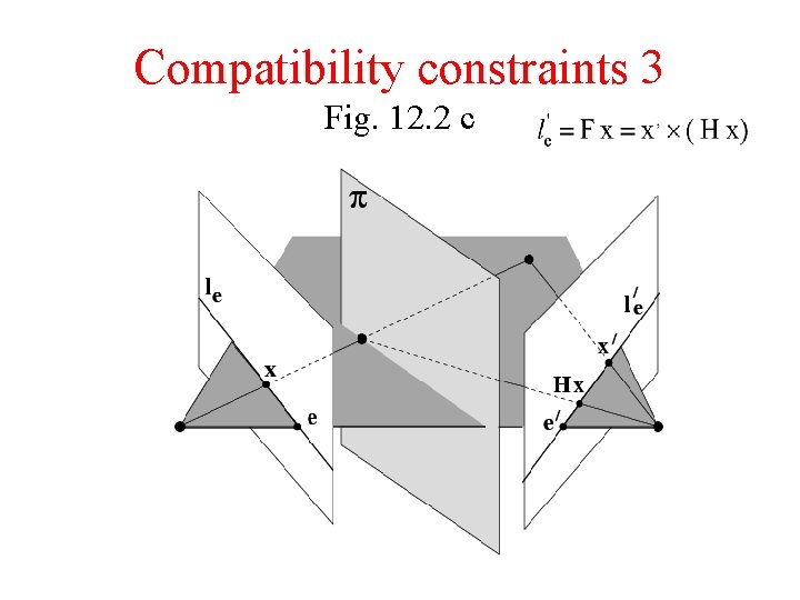
Compatibility constraints 3 Fig. 12. 2 c

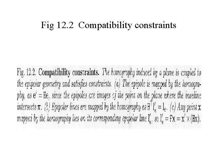
Fig 12. 2 Compatibility constraints

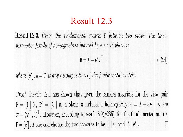
Result 12. 3

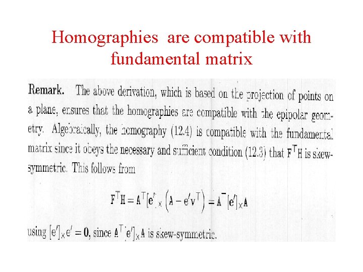
Homographies are compatible with fundamental matrix

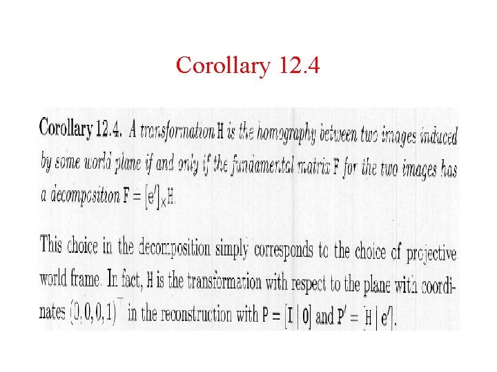
Corollary 12. 4

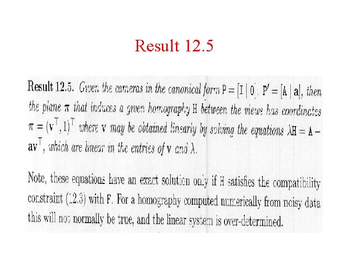
Result 12. 5

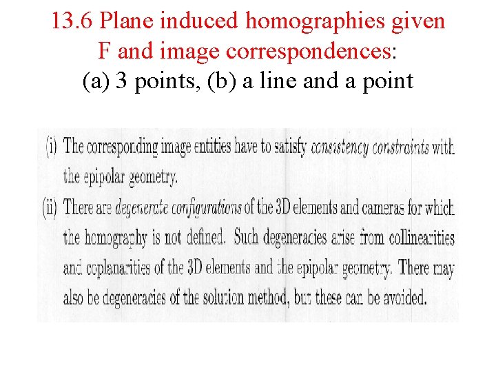
13. 6 Plane induced homographies given F and image correspondences: (a) 3 points, (b) a line and a point

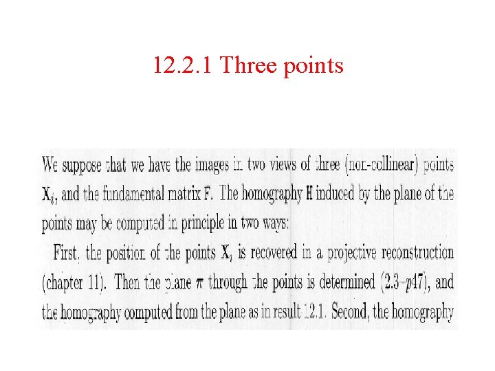
12. 2. 1 Three points

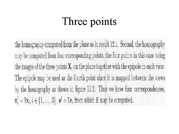
Three points

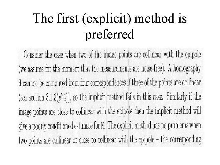
The first (explicit) method is preferred

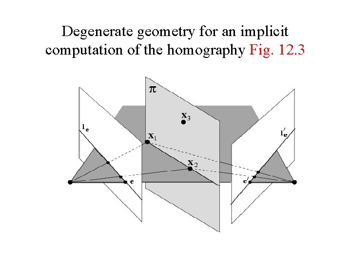
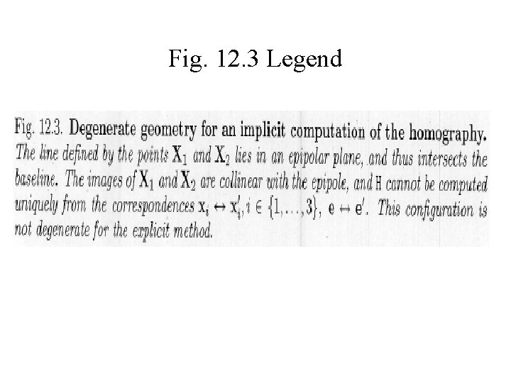
Degenerate geometry for an implicit computation of the homography Fig. 12. 3

Fig. 12. 3 Legend

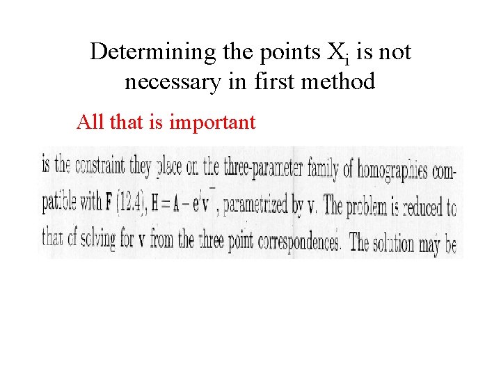
Determining the points Xi is not necessary in first method All that is important

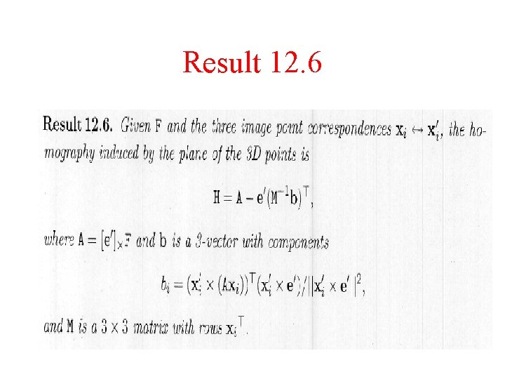
Result 12. 6

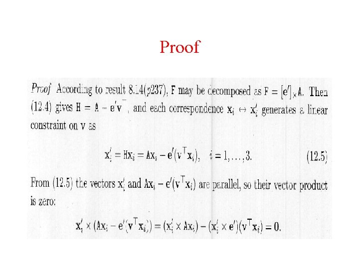
Proof

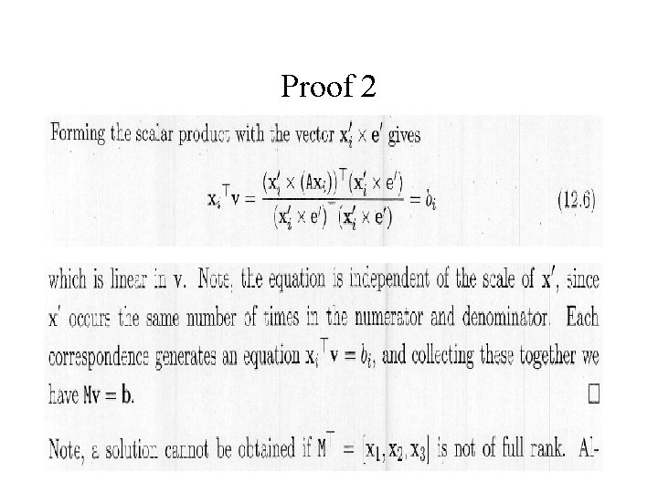
Proof 2

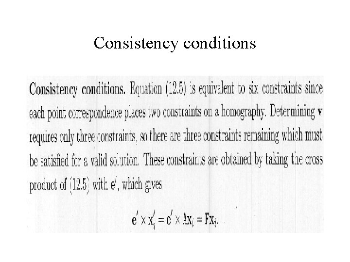
Consistency conditions

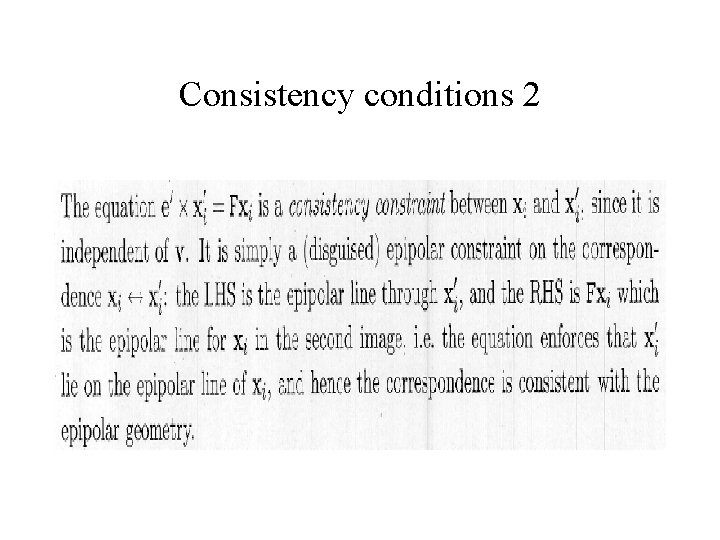
Consistency conditions 2

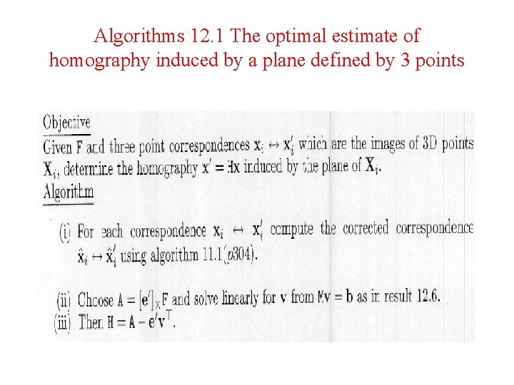
Algorithms 12. 1 The optimal estimate of homography induced by a plane defined by 3 points

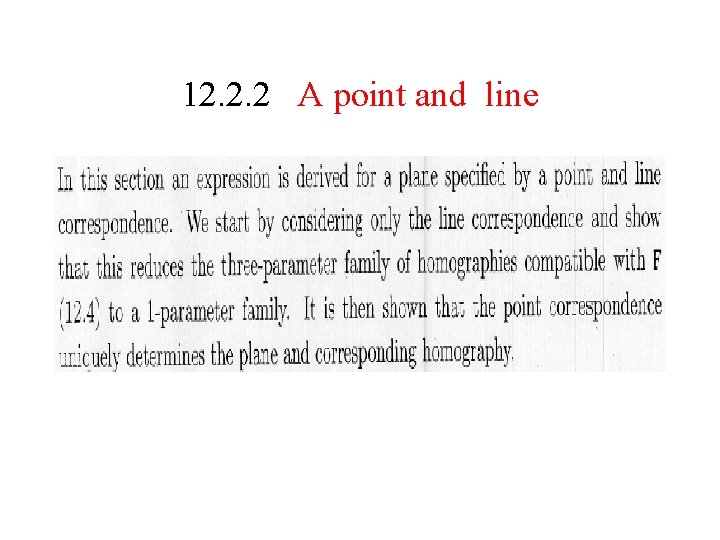
12. 2. 2 A point and line

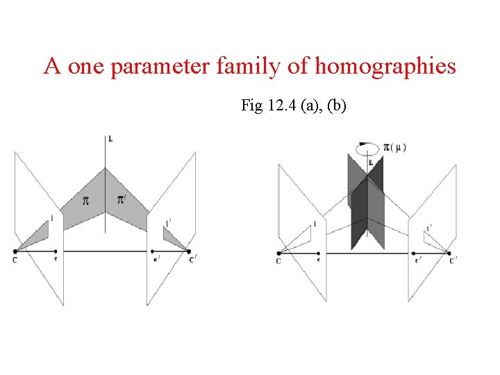
A one parameter family of homographies Fig 12. 4 (a), (b)

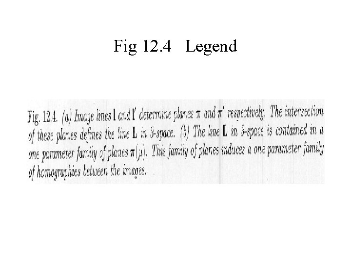
Fig 12. 4 Legend

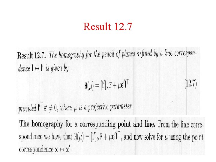
Result 12. 7

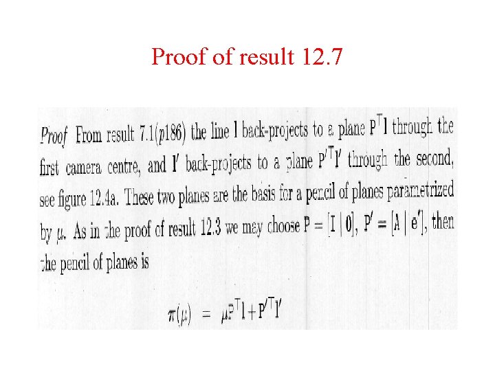
Proof of result 12. 7

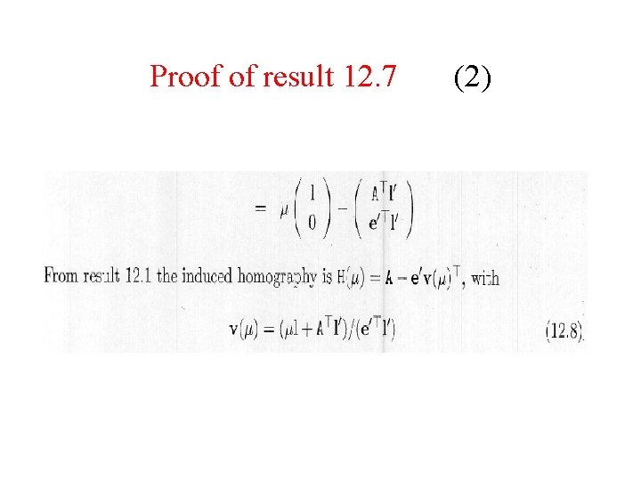
Proof of result 12. 7 (2)

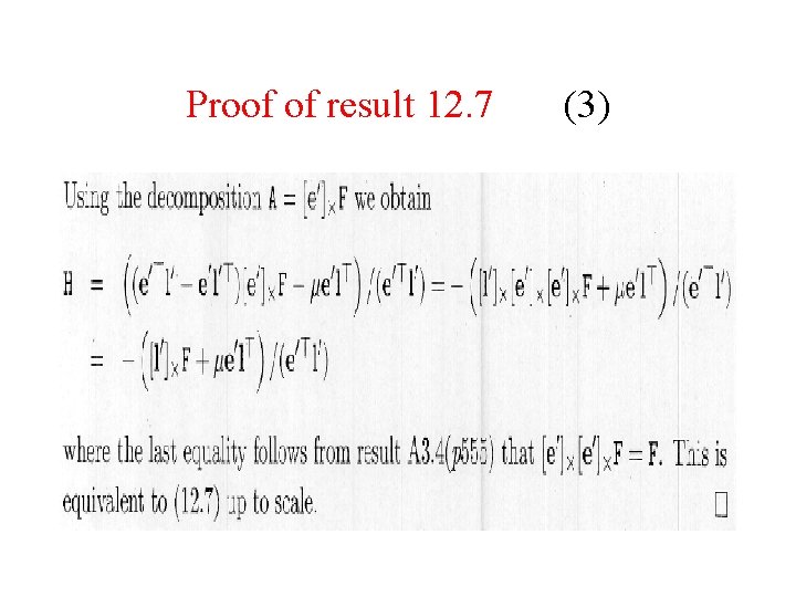
Proof of result 12. 7 (3)

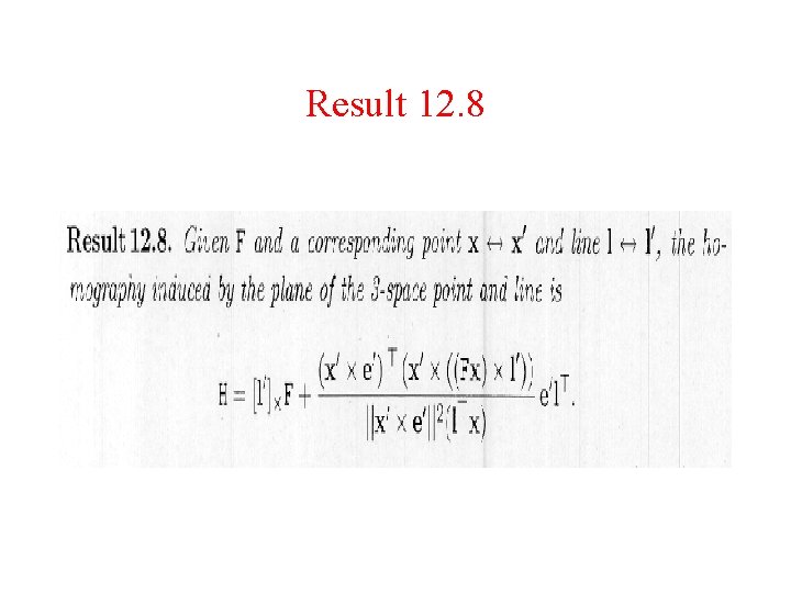
Result 12. 8

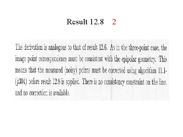
Result 12. 8 2

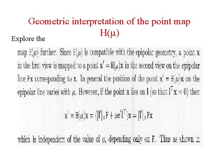
Geometric interpretation of the point map H(m) Explore the

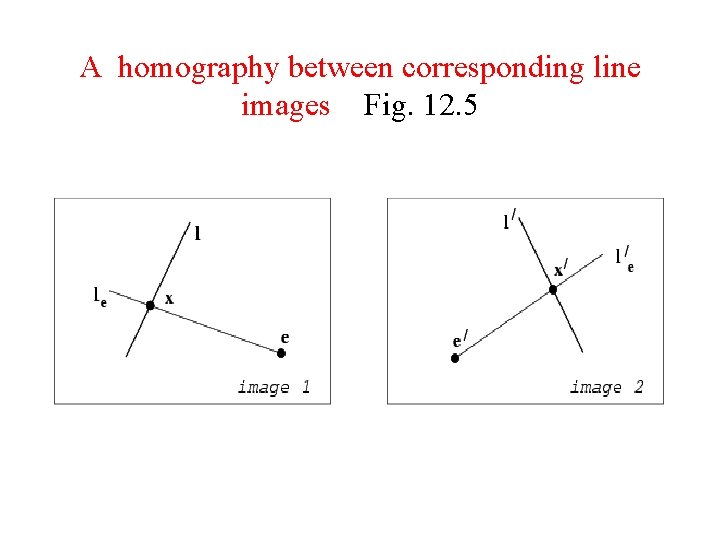
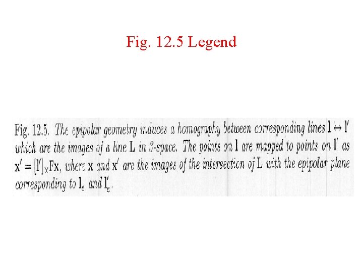
A homography between corresponding line images Fig. 12. 5

Fig. 12. 5 Legend

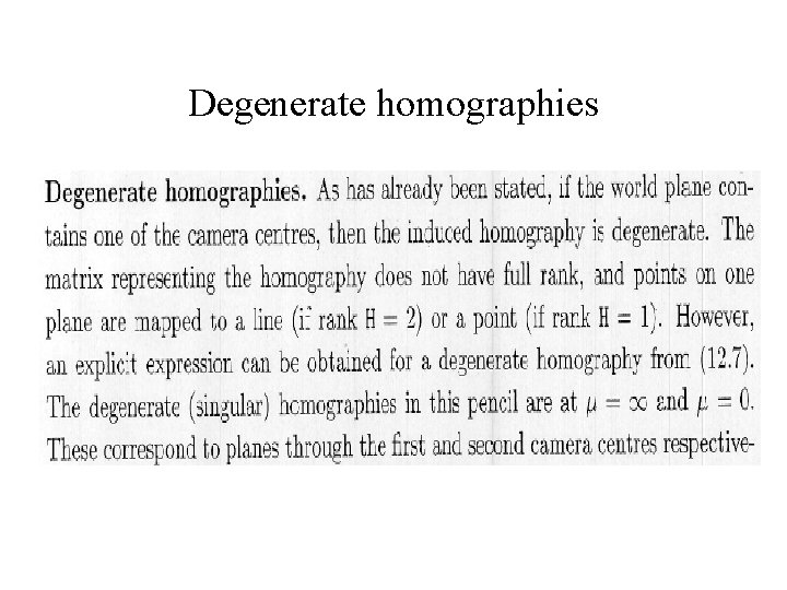
Degenerate homographies

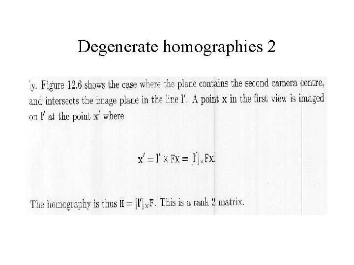
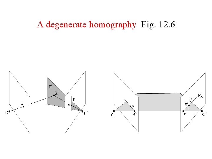
Degenerate homographies 2

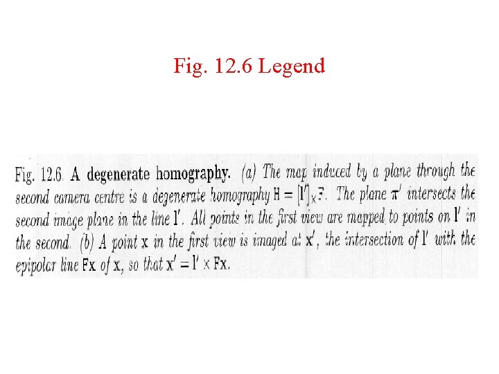
A degenerate homography Fig. 12. 6

Fig. 12. 6 Legend

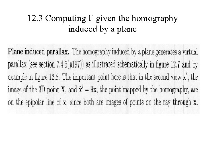
12. 3 Computing F given the homography induced by a plane

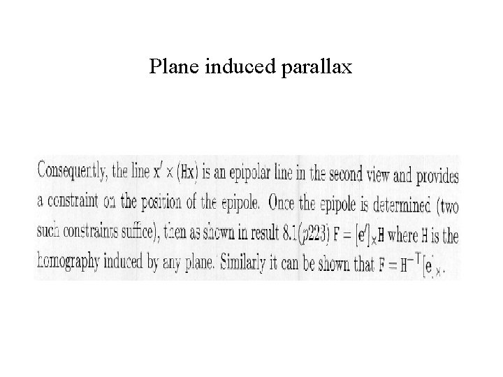
Plane induced parallax

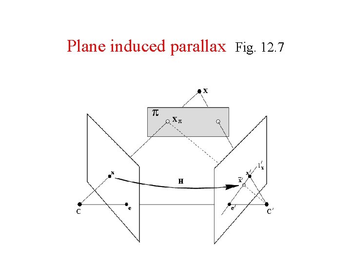
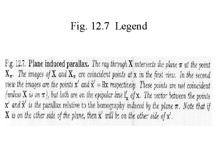
Plane induced parallax Fig. 12. 7

Fig. 12. 7 Legend

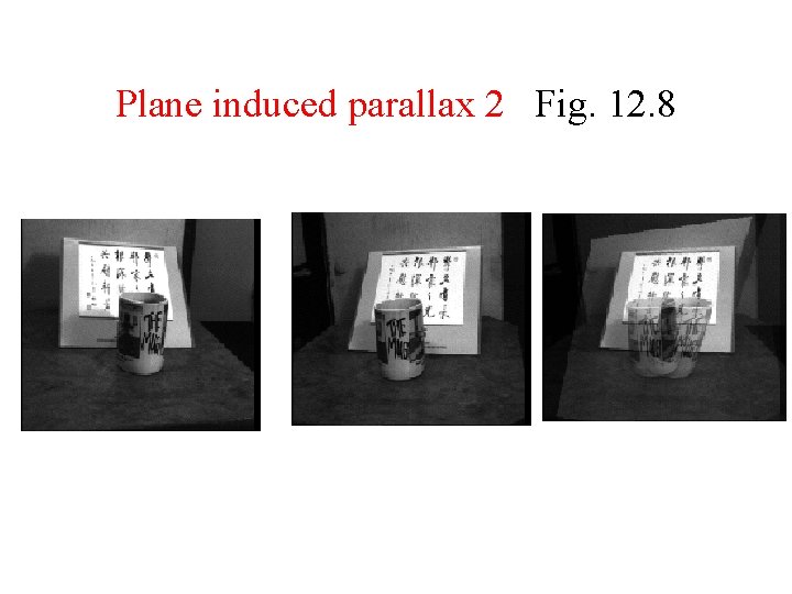
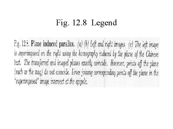
Plane induced parallax 2 Fig. 12. 8

Fig. 12. 8 Legend

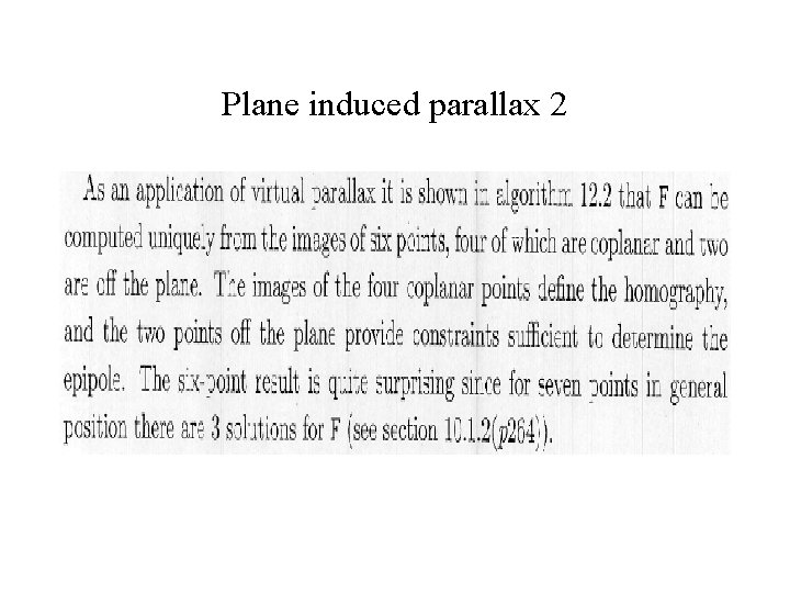
Plane induced parallax 2

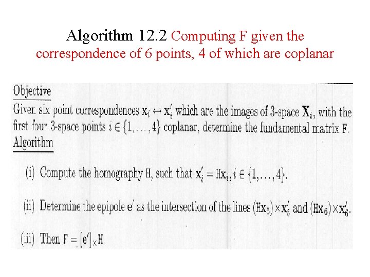
Algorithm 12. 2 Computing F given the correspondence of 6 points, 4 of which are coplanar

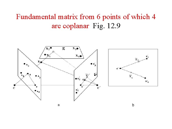
Fundamental matrix from 6 points of which 4 are coplanar Fig. 12. 9

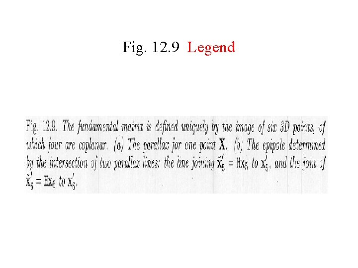
Fig. 12. 9 Legend

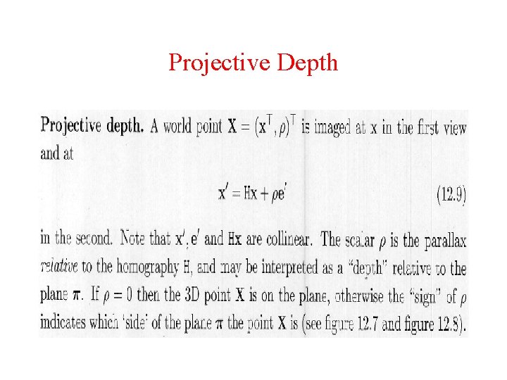
Projective Depth

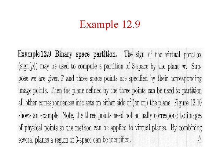
Example 12. 9

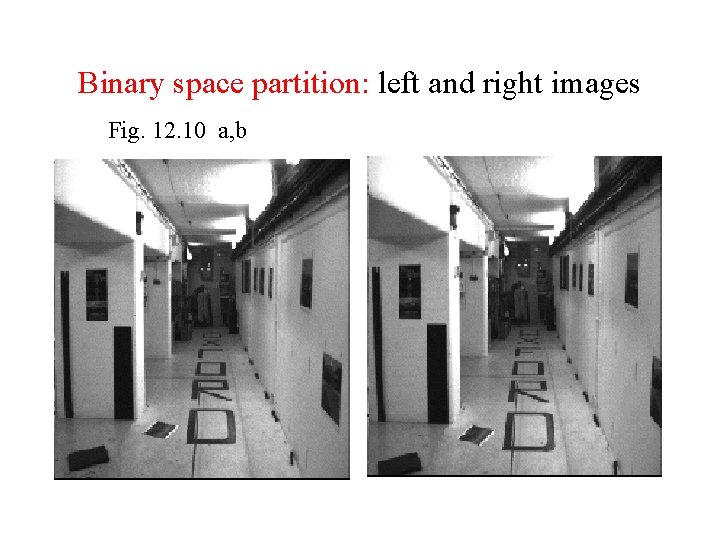
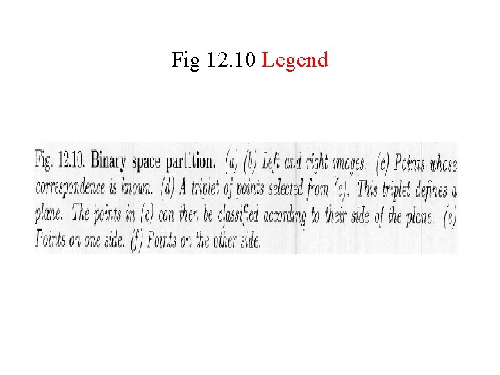
Binary space partition: left and right images Fig. 12. 10 a, b

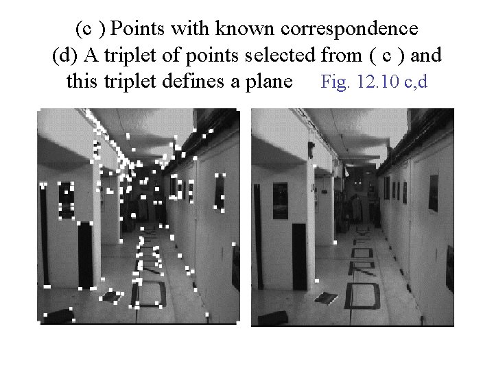
(c ) Points with known correspondence (d) A triplet of points selected from ( c ) and this triplet defines a plane Fig. 12. 10 c, d

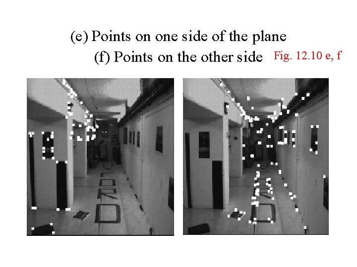
(e) Points on one side of the plane (f) Points on the other side Fig. 12. 10 e, f

Fig 12. 10 Legend

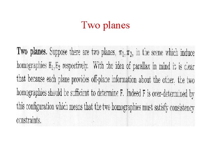
Two planes

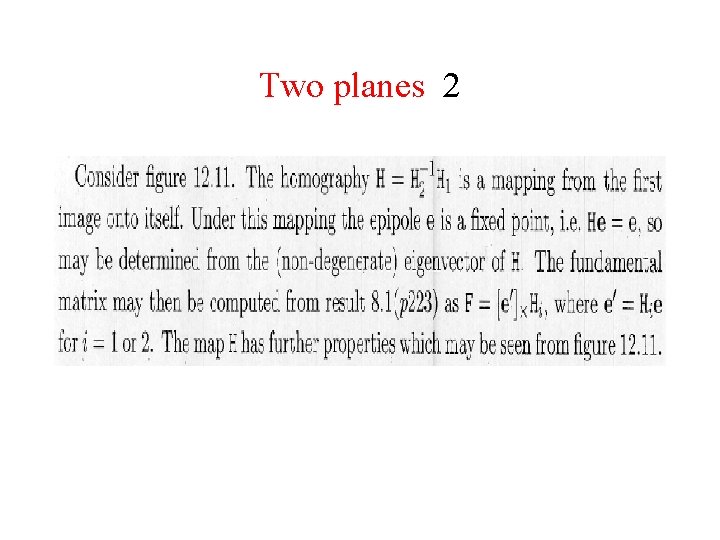
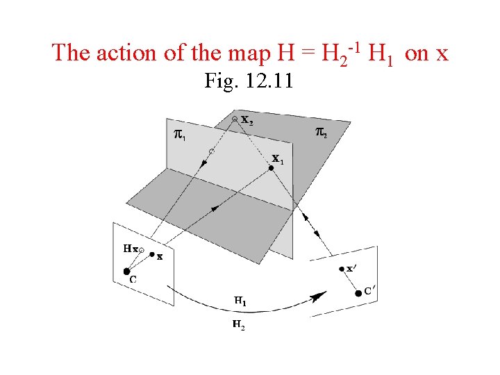
Two planes 2

The action of the map H = H 2 -1 H 1 on x Fig. 12. 11

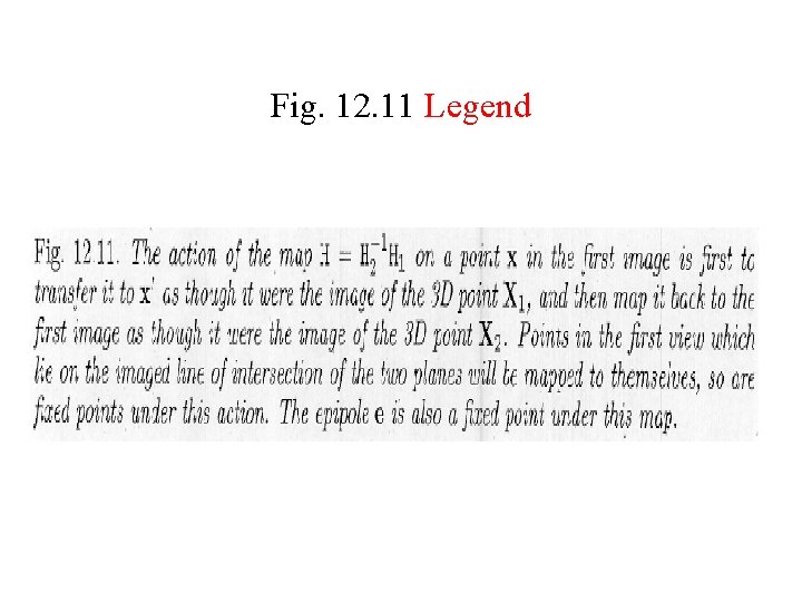
Fig. 12. 11 Legend

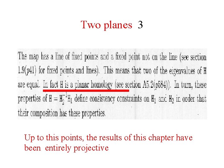
Two planes 3 Up to this points, the results of this chapter have been entirely projective

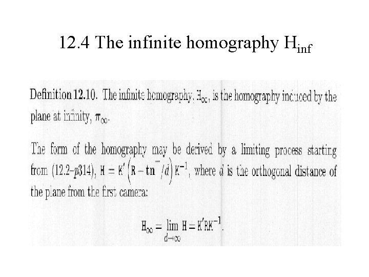
12. 4 The infinite homography Hinf

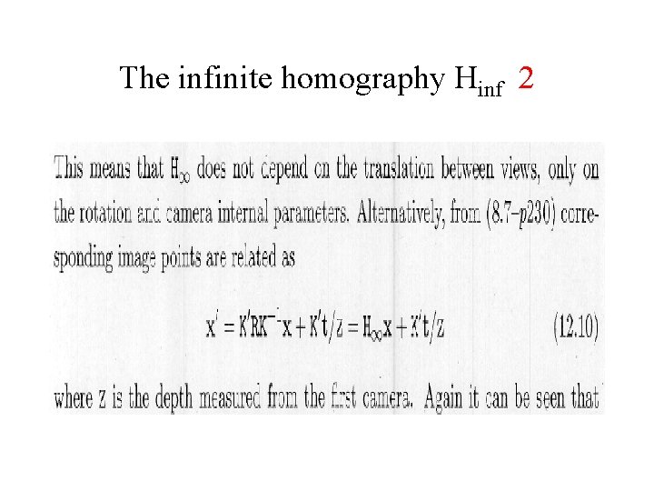
The infinite homography Hinf 2

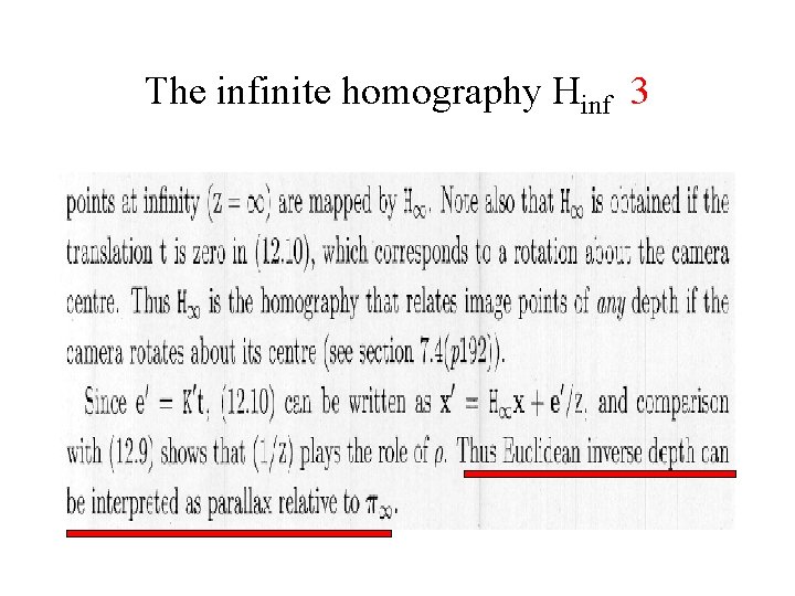
The infinite homography Hinf 3

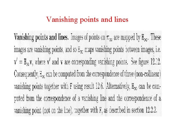
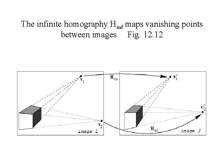
Vanishing points and lines

The infinite homography Hinf maps vanishing points between images Fig. 12

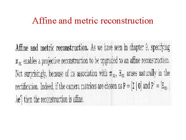
Affine and metric reconstruction

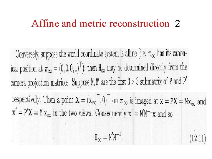
Affine and metric reconstruction 2

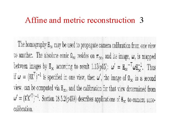
Affine and metric reconstruction 3

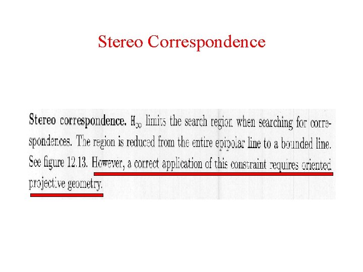
Stereo Correspondence

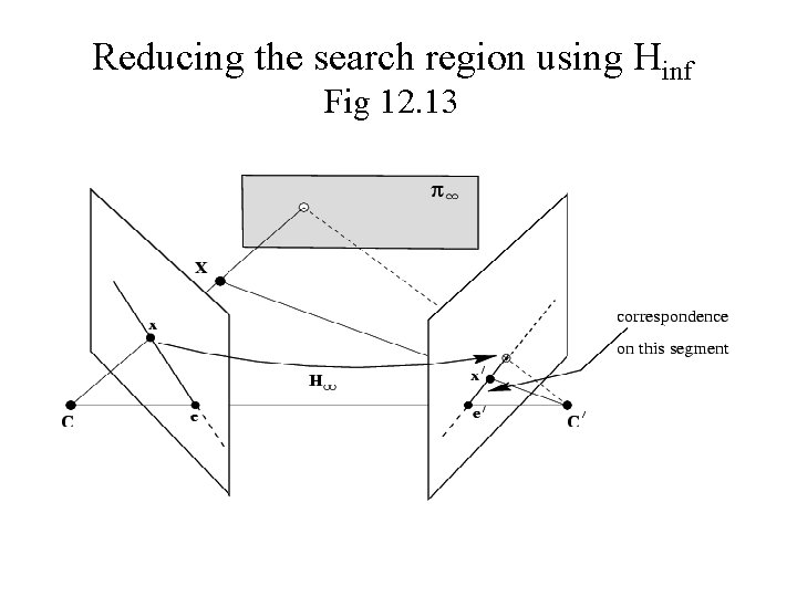
Reducing the search region using Hinf Fig 12. 13

Fig. 12. 13 Legend