Scene Planes and Homographies class 16 Multiple View

Scene Planes and Homographies class 16 Multiple View Geometry Comp 290 -089 Marc Pollefeys

Multiple View Geometry course schedule (subject to change) Jan. 7, 9 Intro & motivation Projective 2 D Geometry Jan. 14, 16 (no class) Projective 2 D Geometry Jan. 21, 23 Projective 3 D Geometry (no class) Jan. 28, 30 Parameter Estimation Feb. 4, 6 Algorithm Evaluation Camera Models Feb. 11, 13 Camera Calibration Single View Geometry Feb. 18, 20 Epipolar Geometry 3 D reconstruction Feb. 25, 27 Fund. Matrix Comp. Rect. & Structure Comp. Planes & Homographies Mar. 18, 20 Trifocal Tensor Three View Reconstruction Mar. 25, 27 Multiple View Geometry Multiple. View Reconstruction Apr. 1, 3 Bundle adjustment Papers Apr. 8, 10 Auto-Calibration Papers Apr. 15, 17 Dynamic Sf. M Papers Apr. 22, 24 Cheirality Project Demos Mar. 4, 6

Two-view geometry Epipolar geometry 3 D reconstruction F-matrix comp. Structure comp.

Planar rectification (standard approach) Bring two views to standard stereo setup (moves epipole to ) (not possible when in/close to image)

Polar rectification (Pollefeys et al. ICCV’ 99) Polar re-parameterization around epipoles Requires only (oriented) epipolar geometry Preserve length of epipolar lines Choose so that no pixels are compressed original image Works for all relative motions Guarantees minimal image size rectified image

polar rectification: example

polar rectification: example

Example: Béguinage of Leuven Does not work with standard Homography-based approaches

Stereo matching • attempt to match every pixel • use additional constraints

Stereo matching Similarity measure (SSD or NCC) Optimal path (dynamic programming ) Constraints • epipolar • ordering • uniqueness • disparity limit • disparity gradient limit Trade-off • Matching cost (data) • Discontinuities (prior) (Cox et al. CVGIP’ 96; Koch’ 96; Falkenhagen´ 97; Van Meerbergen, Vergauwen, Pollefeys, Van. Gool IJCV‘ 02)

Disparity map image I(x, y) Disparity map D(x, y) (x´, y´)=(x+D(x, y) image I´(x´, y´)

Point reconstruction

Line reconstruction doesn‘t work for epipolar plane

Scene planes and homographies plane induces homography between two views

Homography given plane point on plane project in second view

Homography given plane and vice-versa

Calibrated stereo rig

homographies and epipolar geometry points on plane also have to satisfy epipolar geometry! HTF has to be skew-symmetric

homographies and epipolar geometry (pick lp =e’, since e’Te’≠ 0)

Homography also maps epipole

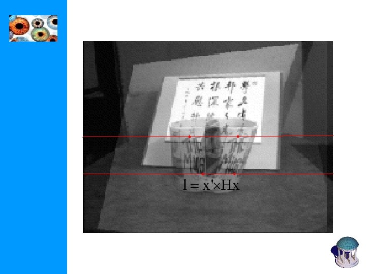
Homography also maps epipolar lines

Compatibility constraint

plane homography given F and 3 points correspondences 1. 2. 3. Method 1: reconstruct explicitly, compute plane through 3 points derive homography 1. 2. Method 2: use epipoles as 4 th correspondence to compute homography

degenerate geometry for an implicit computation of the homography

Estimastion from 3 noisy points (+F) 1. 2. Consistency constraint: points have to be in exact epipolar correspodence 1. Determine MLE points given F and x↔x’ 1. Use implicit 3 D approach (no derivation here)

plane homography given F, a point and a line

application: matching lines 1. (Schmid and Zisserman, CVPR’

epipolar geometry induces point homography on lines

Degenerate homographies

plane induced parallax

6 -point algorithm 1. x 1, x 2, x 3, x 4 in plane, x 5, x 6 out of plane 1. Compute H from x 1, x 2, x 3, x 4

Projective depth 1. 2. r=0 on plane sign of r determines on which side of plane

Binary space partition

Two planes 1. H has fixed point and fixed line

Next class: The Trifocal Tensor