SCATTEROMETER What is a Scatterometer l A scatterometer

SCATTEROMETER

What is a Scatterometer? l A scatterometer is a microwave radar sensor used to measure the reflection or scattering effect produced while scanning the surface of the earth from an aircraft or a satellite.

Background Two kinds of oceanic backscatter Reflection and scattering of a radiance that is normally and obliquely incident on specular and wave-coverd ocean surface

Bragg scatter l Strong oceanic backscatter for incident angles θ as up to 70º λw = λ/2 sinθ where, λw = surface wavelength λ = surface projection of the radar wavelength l For near nadir incidence angles, σ0 ↓ as U ↑ For oblique angles, σ0 ↑ as U ↑ Bragg scatter generated by the interaction between and incident radiance and a specific water wavelength

Backscatter modulation by surface roughness ® Z. Jelenak

Backscatter modulation by surface roughness ® Z. Jelenak

Backscatter modulation by surface roughness ® Z. Jelenak

Backscatter modulation by surface roughness ® Z. Jelenak

Backscatter as a Function of Wind Speed and Incidence Angle Most sensitivity to wind at moderate incidence angles 30°-60° ® Z. Jelenak

Backscatter as a Function of Wind Speed and Incidence Angle Most sensitivity to wind at moderate incidence angles 30°-60° ® Z. Jelenak

Backscatter as a Function of Wind Speed and Incidence Angle Most sensitivity to wind at moderate incidence angles 30°-60° ® Z. Jelenak

Backscatter as a Function of Wind Speed and Incidence Angle Most sensitivity to wind at moderate incidence angles 30°-60° ® Z. Jelenak

Backscatter Sensitivity to Wind Direction 5 m/s ® Z. Jelenak

Backscatter Sensitivity to Wind Direction 20 m/s 15 m/s 10 m/s 5 m/s ® Z. Jelenak

Backscatter Sensitivity to Wind Direction 30 m/s 25 m/s 20 m/s 15 m/s 10 m/s 5 m/s ® Z. Jelenak

Back Scattering Theory l Bragg scattering ¡ Incoming microwave radiation in resonance with short waves (dominant for 30°< q < 70 °) l. B = l/(2 sin(q) l Specular reflection ¡ Ocean facets normal to incident radiation (nonnegligible for q < 30°) l Accuracy of theoretical models ~1 d. B and not adequate l ~ 2 cm (Ku-band) ; l ~ 5 cm (C-band)

History of Scatterometry Observations by radar mounted on aircrafts indicated relationship between surface wind and radar return Scatterometer flown onboard aircraft and Skylab ( S-193) showed good results and hence was planned for Seasat (Seasat-A Satellite Scatterometer : SASS) The first scatterometer flew as part of the Skylab missions in 1973 and 1974 The Seasat-A Satellite Scatterometer (SASS) operated from June to October 1978

History of Scatterometry l A single-swath scatterometer flew on the European Space Agency's Remote Sensing Satellite-1 (ERS-1) mission. l The NASA Scatterometer (NSCAT) which launched aboard Japan's ADEOS-Midori Satellite in August, 1996, was the first dual-swath, scatterometer to fly since Seasat. From September 1996 when the instrument was first turned on, until premature termination of the mission due to satellite power loss in June 1997, The NSCAT mission proved so successful, that plans for a follow-on mission were accelerated to minimize the gap in the scatterometer wind database. l The Quik. SCAT mission launched Sea. Winds in June 1999

Table of Satellite Scatterometers Short Background Period in Service Spatial Resolution Scan Characteristics Operational Frequency Sea. Sat-A 1978/7/7 - Scatterometer 1978/10/10 50 km with two sided, 100 km double swath spacing Ku band (14. 6 GHz) ERS-1 1991/7 - Scatterometer 1997/5/21 50 km one sided, single swath C band (5. 3 GHz) ERS-2 1997/5/21 - Scatterometer current 50 km one sided, single swath C band (5. 3 GHz) NSCAT 1996/9/15 - 1997/6/30 25 km, and two sided, 50 km double swath Ku band (13. 995 GHz) Sea. Winds on Quik. SCAT 1999/7/19 - current 25 km conical scan, one wide swath Ku band (13. 4 GHz) Sea. Winds on ADEOS II Launch Date 25 x 6 km Dec. 2001 conical scan one wide swath Ku band (13. 4 GHz)

EUMETSAT l The European Space Agency has its own scatterometers in orbit, such as Envisat. It is now running on a backup transmitter and have other problems, this satellite could fail at any moment. l Now ASCAT on board METOP provides sea surface winds

ESCAT refers to the Active Microwave Instrument (AMI) scatterometer aboard the European Space Agency's (ESA's) Earth Remote Sensing (ERS)-1 and -2 satellites. The advanced scatterometer (ASCAT) on the European Space Agency's Met Operational (Met. Op) platforms are the follow-on to European wind scatterometers. Metop -1 was launched on 19 Oct 2006 The NASA Scatterometer (NSCAT) flew on the Japanese Aerospace Exploration (JAXA, formerly known as NASDA) Advanced Earth Observing Satellite (ADEOS-I) The Sea. Winds scatterometer flies on NASA's Quick Scatterometer (Quik. SCAT) satellite. A similar scatterometer, Sea. Winds-II, flew on JAXA's ADEOS-II satellite before a power failure terminated the mission.

Quik. SCAT l The Sea. Winds on Quik. SCAT mission is a "quick recovery" mission to fill the gap created by the loss of data from the NASA Scatterometer (NSCAT), when the satellite it was flying on lost power in June 1997. The Sea. Winds instrument on the Quik. SCAT satellite is a specialized microwave radar that measures near-surface wind speed and direction under all weather and cloud conditions over Earth's oceans l In light of the 2003 failure of the ADEOS II satellite that was meant to succeed the NSCAT, Quick. SCAT is currently the only US-owned instrument in orbit that measures surface winds over the oceans

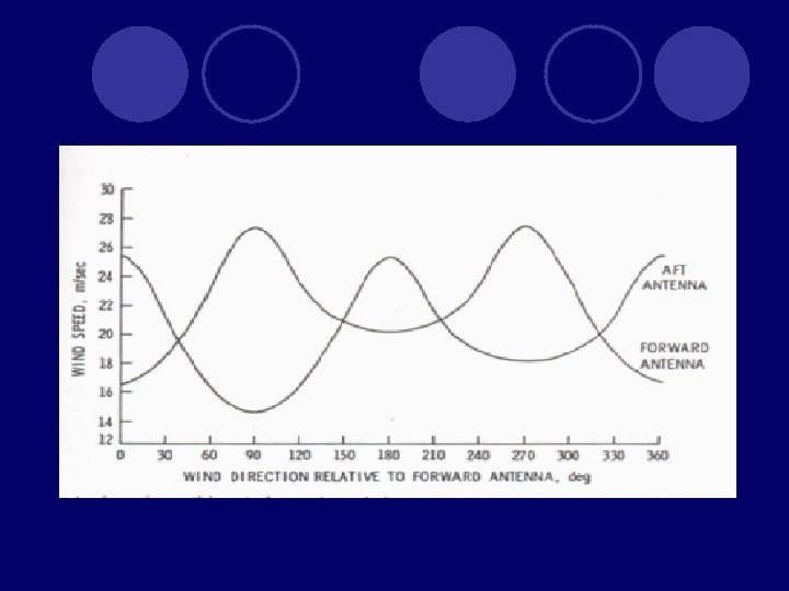
Principle Of Scatteromery The estimation of wind velocity from scatterometers require multiple co-located measurement of backscatter from different azimuth angles The multiple azimuth viewing is met using either fan beam antennas or scanning spot beams Earlier instruments relied on fan beam antennas The fan beam antenna configuration is essentially a side looking radar However, since the measurements have to be made at different zenith angles, multiple antennas oriented at different angles is used A given surface is first viewed by the forward antenna and later by the aft antenna Thus o measurement of the same place is provided by two azimuth angles separated by 90

Sea Surface Roughness - Oblique-viewing microwave radiometers Microwave scatterometer is based on the principle of the resonant Bragg scattering. For a smooth surface, oblique viewing of the surface with active radar yields virtually no return. If the surface is rough, significant backscatter occurs.

Bragg’s Resonance

Sea Surface Roughness - Oblique-viewing microwave radiometers Tropical cyclone observed by Quik. SCAT in June 2007.

SEASAT-A SCATTEROMETER ANTENNA PATTERN l SASS uses four fan beam antennas — two on either sides of the sub -satellite track l The two antennas on each side are aligned so that they are pointed 45° and 135° relative to the spacecraft flight direction

Waves induces waves of all wavelengths on the sea surface Waves that are near the wavelength of 1. 75 cm backscatter radiation through Bragg Scattering As SASS wavelength is 2 cm, capillary waves are responsible for backscatter Many parameters influence o (wind speed, polarisation, viewing angle, relative azimuth between the radar beam and wind direction etc. ) Max backscatter occurs in the upwind and downwind directions and minimum near the cross wind direction To account for the wind shear in the boundary layer, wind speed U taken for calculations is the 19. 5 m neutral stability wind U is calculated from boundary layer model and one of the input for the model is the height of the anemometer

MODEL FUNCTIONS l Empirical relationship between o and wind vector l The Model functions available for Ku and C bands are known as SASS-1 and CMOD 4. l SASS-1 Model functions o = 10 G(θ, , p) + 10 H(θ, , p). log(W) Where θ – incident angle , - aspect angle G and H are model functions. The tabulated values of G and H were determined empirically using pre launch aircraft and post launch SASS observations of o

MODEL FUNCTIONS l Suppose SASS has only two observations, then we have two equations 1 o = 10 G(θ 1, 1, p 1) + 10 H(θ 1, 1, p 1). log(W) 2 o = 10 G(θ 2, 1+90, p 2)+10 H(θ 2, 1+90, p 2). log(W) There are two non linear Eqns in two unknowns W and 1. They can be solved by plotting W versus 1. The two eqns give two curves Since o is max. at up and downwind and minimum at cross winds, the curve has two maxima and two minima and they are separated by 90 The points where the curves intersect are the solutions (aliases) One of them represent the true wind To reduce the no. of aliases the next generation scatterometers had two additional antennas to reduce the no. of aliases

Justifications for making measurements at various azimuth angles

NSCAT ANTENNA PATTERN l Two sets of antennae covering both sides of the track l Each set has three antennae covering a swath of 800 Km l Polarisation of MW radiation emitted and received by the mid beam is both vertical (VV) and horizontal(HH) l For others only VV polarisation is used

PENCIL BEAM ANTENNA PATTERN l Consists of two off nadir beams inner and outer l Each point in the inner swath is scanned twice by the inner and twice by outer beam l These four enable retrieval with better accuracy

ADVANTAGES OF PENCIL BEAM SCATTEROMETER High o measurement accuracy due concentrated pencil beam High directional accuracy as each point is viewed four times No nadir gaps Simplified Model Functions: Only two incident angle Easier signal processing Smaller in size

RETRIEVAL ALGORITHMS Radar backscatter has a harmonic dependence on wind direction which results in multiple solutions Two retrieval algorithms are used • • Prioritisation Wind ambiguity removal The retrieval algorithm give multiple solutions along with prioritisation For a noise free signal, highest priority solution gives the true wind vector The first two prioritised winds invariably give the correct wind vector

Retrieval Algorithm for Prioritisation The average and SD of wind speed is calculated from the entire range of aspect angles Then, the minima of the SD of the wind speeds are searched along the aspect angle The solution having the minimum SD is selected as the first priority solution and the next lowest as the second solution and so on. These are now need to be cleared of directional ambiguity

EXAMBLE OF PRIORITISED WIND VECTOR SOLUTION FOR NOISE FREE o CMOD 4 Model Function for ERS! Forward SD Mid Mean Aft

MEDIAN FILTER How It Works Like the mean filter, the median filter considers each pixel in the image in turn and looks at its nearby neighbors to decide whether or not it is representative of its surroundings. Instead of simply replacing the pixel value with the mean of neighboring pixel values, it replaces it with the median of those values. The median is calculated by first sorting all the pixel values from the surrounding neighborhood into numerical order and then replacing the pixel being considered with the middle pixel value. (If the neighborhood under consideration contains an even number of pixels, the average of the two middle pixel values is used. ) Figure 1 illustrates an example calculation.

l By calculating the median value of a neighborhood rather than the mean filter, the median filter has two main advantages over the mean filter: l The median is a more robust average than the mean and so a single very unrepresentative pixel in a neighborhood will not affect the median value significantly. l Since the median value must actually be the value of one of the pixels in the neighborhood, the median filter does not create new unrealistic pixel values when the filter straddles an edge. For this reason the median filter is much better at preserving sharp edges than the mean filter.

Figure 1 Calculating the median value of a pixel neighborhood. As can be seen, the central pixel value of 150 is rather unrepresentative of the surrounding pixels and is replaced with the median value: 124. A 3× 3 square neighborhood is used here --- larger neighborhoods will produce more severe smoothing.

This figure shows a typical region with each of the wind ambiguities displayed at each cell. Blue is the first (most likely) ambiguity, red is the second, green the third and aqua the fourth. In order to determine an estimate of the wind across the entire swath, an ambiguity selection algorithm is needed.

The Point-wise Median Filter l In order to select the proper ambiguity, we assume that the estimates are correlated from one cell to the next. In other words, we assume that the wind is unlikely to shift radically from one cell to the next. Using this assumption, we may use a variety of techniques to select a single ambiguity at each wvc. l A common technique used to correlate the estimates is based on the point-wise median filter. This method does not alter any of the wind estimates generated; rather is selects between the ambiguities at each cell. Like median filters used in image processing, the point-wise median filter attempts to preserve edges and avoid blurring. l The entire swath is initialized to the first ambiguity. For each cell in the swath, a 7 -cell window is generated around the cell in question, and an average of all of the wind vectors is taken. The ambiguity closest to this windowed average is selected. This process is repeated until there are no more changes (or until a maximum number of iterations is achieved).

DIRECTIONAL AMBIGUITY REMOVAL Uses two highest priority wind vectors In ERS-1 scatterometer antenna configuration more than half of first priority winds represent the true winds and the remaining solutions are opposite to the true wind Median Filtering approach is used to remove the ambiguity- Trend or consensus of highest priority directions is derived over median window For this, the highest priority vectors are resolved in to zonal and meridional components. With a moving window of optimal size, medians of both scalars at each data location are determined

DIRECTIONAL AMBIGUITY REMOVAL The median scalar yield median wind direction at each data location which is used to select the direction out of the two highest prioritised winds The procedure is followed for entire satellite pass to select the solution nearer to the median direction At this stage the winds mostly resemble the true wind field. The direction closer to the median direction is retained and not replaced by the median direction(Gohil 1992) If the data is noisy then some ambiguities may still prevail and may be removed by using a supplementary method.

RESULTS OF ERS-1 l Ocean surface winds for the period Aug 1992 - Jul 1993 l ERS-1 data used to prepare monthly and fortnightly averaged windfields l Strong SWly winds noticed off Somali coast l Branching of winds over Arabian sea noticed l Intensity is weak in May and strong in Jun l Data compared with near co located data taken from ships( within 6 hrs and 0. 5 deg) at 47 locations l Showed god agreement with SAT instrument specifications of 2 m/sec or 10% (whichever is more) l Underestimated when spped was less than 5 m/sec and over estimation when spped was more than 5 m/ses l The RMS deviation of 20 deg was observed as against the

l ADEOS: Advanced Earth Observing Satellite l AMI: Active Microwave Instrument l DAAC: Distributed Active Archive Center l ERS-1/2: European Remote Sensing Satellite l ESCAT: AMI scatterometer on ERS-1/2 satellites l NASA: National Aeronautics and Space Administration l NSCAT: NASA Scatterometer l Quik. SCAT: Quick Scatterometer l SASS: Seasat-A Scatterometer System

Where to Get Scatterometer Data l NRL Monterey http: //kauai. nrlmry. navy. mil: 80/sat-bin/tc_home l NOAA/NESDIS Quik. SCAT http: //manati. wwb. noaa. gov/quikscat Storms page – includes ambiguities: http: //manati. wwb. noaa. gov/cgi-bin/qscat_storm. pl Alternative NOAA site, with SSMI wind speeds: http: //polar. wwb. noaa. gov/winds/globdata. html l FNMOC http: //www. fnmoc. navy. mil/PUBLIC l Remote Sensing Systems http: //www. ssmi. com APSATS 2002, Melbourne Australia

Differences l Wind retrieval RSS uses KU-2000 wind retrieval method Others use Quik. SCAT 1 wind retrieval method l Rain Flags Generally Multidimensional Histogram (MUDH) procedure – a statistical method based on “noisiness” of data RSS has similar approach though it is less conservative and hence rain affected areas are often smaller APSATS 2002, Melbourne Australia

Ambiguity Selection l NOAA/NESDIS use rain flagged data in ambiguity selection process l FNMOC does not – rain flagged data is put in “as is” after ambiguity removal. APSATS 2002, Melbourne Australia

What is it GOOD for? l Detection of circulations and determination of windspeeds. X 09/04/02 0922 Z TC Bonnie in its early stages. Note gales on the southern side. APSATS 2002, Melbourne Australia

Small system (X) could be followed for 3 days --no help from NWP model 20 S O X 170 W O X 25 Jan 1800 Z X O 26 Jan 0517 Z 26 Jan 1800 Z 170 W 160 W O X O APSATS 2002, Melbourne Australia 27 Jan 1712 Z 28 Jan 0427 Z

What is it GOOD for? l Location of fronts/troughs. l Wind speeds in data sparse areas. APSATS 2002, Melbourne Australia

When is it BAD? l Edge of swath (~ 7 wind vector cells) l Rain effects l Sensitivity to errors in NWP l Practical wind regime 5 -45 m/s very light and very strong winds) l Resolution (25 km) (problems with both – impact in tight gradients l Ambiguity Removal Process and rain flag process can affect final solution APSATS 2002, Melbourne Australia

Edge Problems Along the whole edge… FNMOC DISPLAY APSATS 2002, Melbourne Australia or small portion…

Rain Flags RSS TC Chris 05/02/02 0937 Z Rain flagged areas APSATS 2002, Melbourne Australia NRL

Typical Rain Patterns Rain effects: Cross swath vectors Higher wind speeds Some intense rain not flagged APSATS 2002, Melbourne Australia RSS slide

Rain Effects One or two bad wind solutions may affect neighboring wind vector cells through buddychecking system causing a ‘rain contagion’ effect. TC Chris 05/02/02 0937 Z Direction of swath Rain block – direction perpendicular to swath Do not use direction – speed may be OK APSATS 2002, Melbourne Australia

Streamlines TC Chris 03/02/02 0914 Z Beware of winds perpendicular to the swath, even when they are not flagged X Look for non-rain flagged winds APSATS 2002, Melbourne Australia

Model initialisation errors In this case, poor model initialization combined with a lower skill nadir position, picks proper wind speed, but NO circulation center 20/2356 Z AVN 19/12 Z tau 24 (Light winds? ) -----low skill 10 S c ? c 10 S ? 20 S Max Wind 55 KTS TC Paul 20 S APSATS 2002, Melbourne Australia

http: //manati. star. nesdis. noaa. gov/datasets/ERS 2 Data. php

ASCAT WINDS

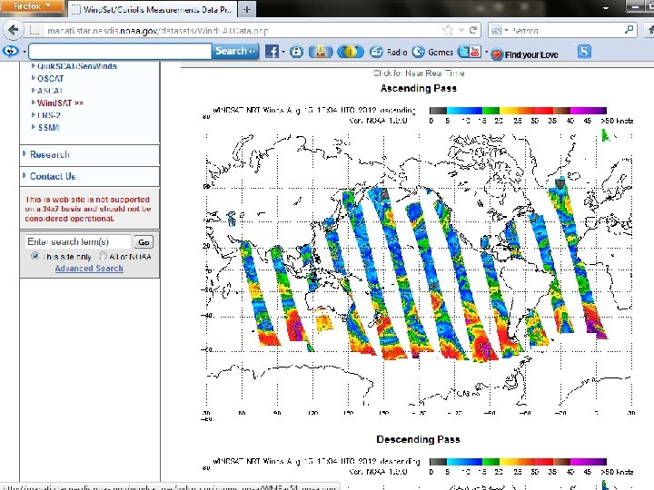
ASCAT WINDS OVER INDIA : 13 AUG 12

ASCAT WINDS OVER INDIA : 13 AUG 12

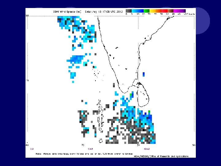
OCEANSAT 2 WINDS: 13 AUG 12

WINDSAT is a joint NOAA Integrated Program Office /Department of Defense/NASA demonstration project, intended to measure ocean surface wind speed and wind direction from space using a polarimetric radiometer. It was launched aboard the Coriolis satellite by a Titan II rocket on 6 January 2003 into a 830 -km 98. 7 -degree orbit, and is designed for a three-year lifetime.

WINDSAT l Wind. Sat is a satellite-based polarimetric microwave radiometer developed by the Naval Research Laboratory Remote Sensing Division, the Naval Center for Space Technology, and the National Polar-orbiting Operational Environmental Satellite System (NPOESS) Integrated Program Office (IPO). l It was launched in January 2003 aboard the joint Do. D/Navy platform Coriolis, with a planned 3 -year life. Despite its extended lifespan, it continues to function quite well. l Wind. Sat measures the ocean surface wind vector, as well as cloud liquid water, sea surface temperature, total precipitable water, and rain rate (over water only). Derived products include soil moisture and sea ice.

l The Navy, NOAA, and UK Met Office frequently use Wind. Sat data in several operational forecast models. l Coriolis is sun-synchronous (1800 UTC equator crossing time) and Wind. Sat has a swath width of ~1000 km, with a resolution is ~50 km. l Wind. Sat data had always been a secondary wind observation with Quik. SCAT (launched 1999) as the primary source, because of its better resolution and accuracy. However, when Quik. SCAT failed in 2009, NRL researchers were encouraged to push their improved Wind. Sat algorithm into operations.

Conclusions l Provides coverage over data sparse areas l Wind speeds generally good – useful for areas of gales etc l Use the data if it makes sense l Be aware of low skill areas and different ambiguity removal processes (compare!) l Do not use in isolation APSATS 2002, Melbourne Australia