Scaling BackPropagation by Parallel Scan Algorithm Shang Wang

Scaling Back-Propagation by Parallel Scan Algorithm Shang Wang 1, 2, Yifan Bai 1, Gennady Pekhimenko 1, 2 1 2

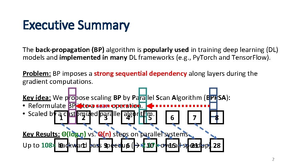
Executive Summary The back-propagation (BP) algorithm is popularly used in training deep learning (DL) models and implemented in many DL frameworks (e. g. , Py. Torch and Tensor. Flow). Problem: BP imposes a strong sequential dependency along layers during the gradient computations. Key idea: We propose scaling BP by Parallel Scan Algorithm (BPPSA): • Reformulate BP into a scan operation. • Scaled by a customized parallel algorithm. 1 2 3 4 5 6 7 8 Key Results: Θ(log n) vs. Θ(n) steps on parallel systems. Up to 108× backward 0 1 pass speedup 3 6 (→ 2. 17× 10 overall 15 speedup). 21 28 2

1 Back-propagation (BP) Everywhere 1 Rumelhart et al. “Learning representations by back-propagating 3 errors. ”, Nature (1986)

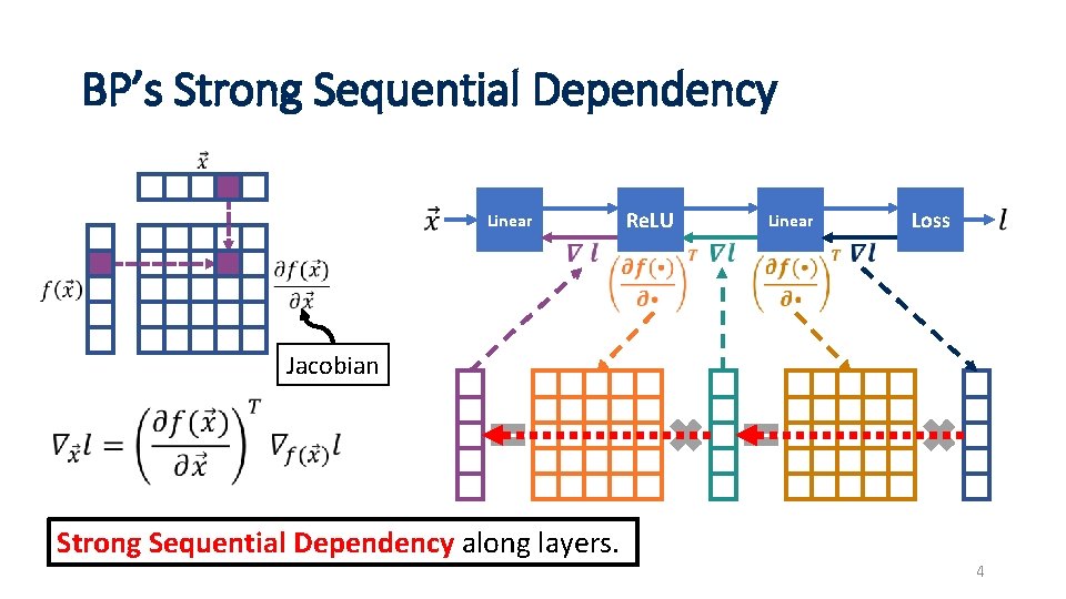
BP’s Strong Sequential Dependency Linear Re. LU Linear Loss Jacobian Strong Sequential Dependency along layers. 4

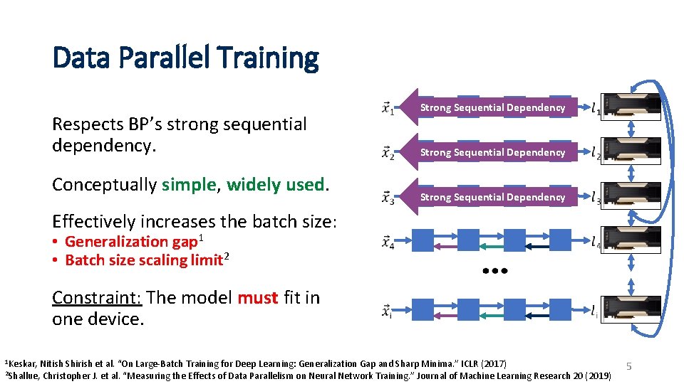
Data Parallel Training Respects BP’s strong sequential dependency. Conceptually simple, widely used. Strong Sequential Dependency Effectively increases the batch size: • Generalization gap 1 • Batch size scaling limit 2 Constraint: The model must fit in one device. 1 Keskar, Nitish Shirish et al. “On Large-Batch Training for Deep Learning: Generalization Gap and Sharp Minima. ” ICLR (2017) 2 Shallue, Christopher J. et al. “Measuring the Effects of Data Parallelism on Neural Network Training. ” Journal of Machine Learning Research 20 (2019) 5

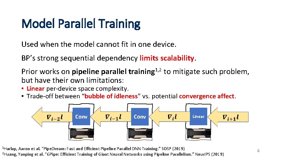
Model Parallel Training Used when the model cannot fit in one device. BP’s strong sequential dependency limits scalability. Prior works on pipeline parallel training 1, 2 to mitigate such problem, but have their own limitations: • Linear per-device space complexity. • Trade-off between “bubble of idleness” vs. potential convergence affect. Conv 1 Harlap, 2 Huang, Conv Linear Aaron et al. “Pipe. Dream: Fast and Efficient Pipeline Parallel DNN Training. ” SOSP (2019) Yanping et al. “GPipe: Efficient Training of Giant Neural Networks using Pipeline Parallelism. ” Neur. IPS (2019) 6

Rethinking BP from an Algorithm Perspective Prior Works • Problems with strong sequential dependency were studied in the past (80’), but in a much simpler context. BP • We propose scaling Back-Propagation by Parallel Scan Algorithm (BPPSA): • Reformulate BP as a scan operation. • Scale BP by a customized Blelloch Scan algorithm. • Leverage sparsity in the Jacobians. BP BPPSA 7

What is a Scan 1 Operation? Binary, associative operator: + Identity: 0 Input sequence: 1 2 3 4 5 6 7 8 Exclusive scan: 0 1 3 6 10 15 21 28 Compute partial reductions at each step of the sequence. 1 Blelloch, Guy E. ”Prefix sums and their applications”. Technical Report (1990) 8

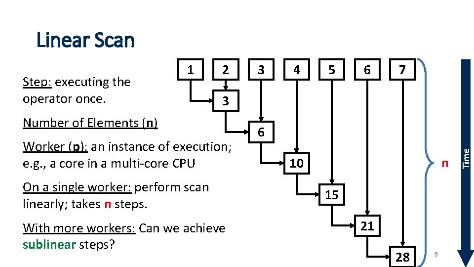
Linear Scan 2 3 4 5 6 7 3 Number of Elements (n) Worker (p): an instance of execution; e. g. , a core in a multi-core CPU On a single worker: perform scan linearly; takes n steps. With more workers: Can we achieve sublinear steps? 6 n 10 15 21 28 9 Time Step: executing the operator once. 1

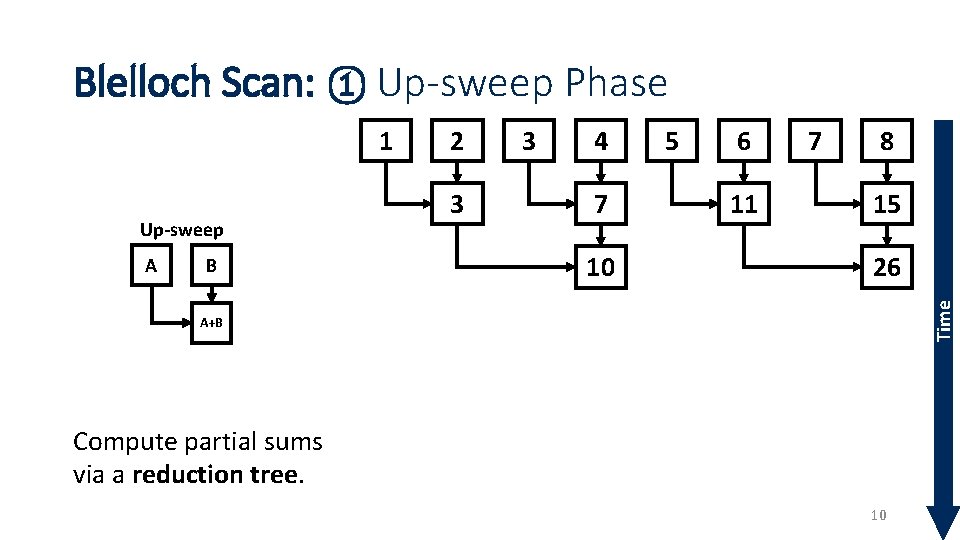
Blelloch Scan: ① Up-sweep Phase Up-sweep A B 2 3 3 4 7 10 5 6 11 7 8 15 26 Time 1 A+B Compute partial sums via a reduction tree. 10

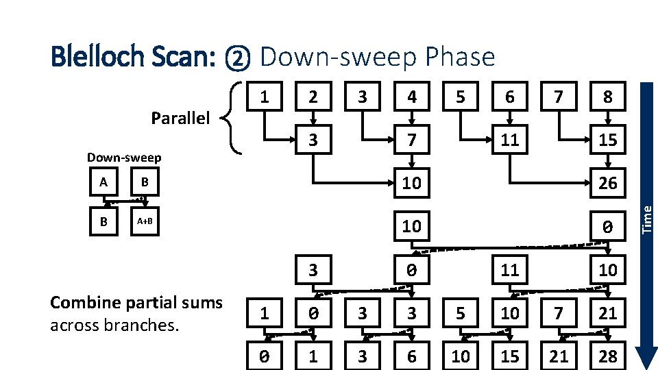
Blelloch Scan: ② Down-sweep Phase 2 3 3 Down-sweep 4 5 7 6 7 11 8 15 A B 10 26 B A+B 10 0 3 Combine partial sums across branches. 11 0 10 1 0 3 3 5 10 7 0 1 3 6 10 15 21 21 28 11 Time Parallel 1

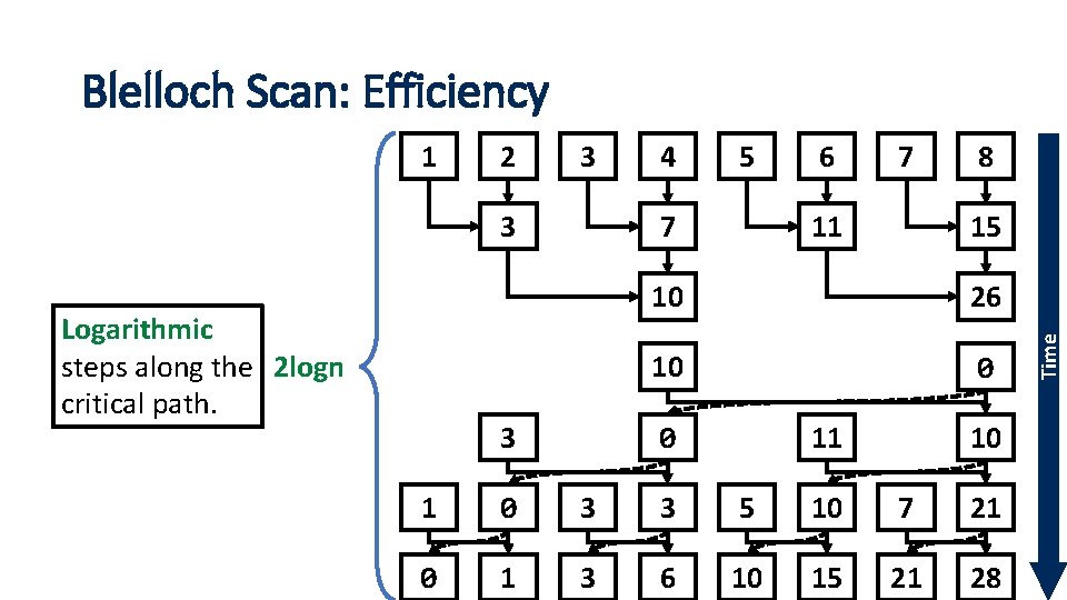
Blelloch Scan: Efficiency 2 3 3 Logarithmic steps along the 2 logn critical path. 4 5 7 3 6 7 11 8 15 10 26 10 0 11 0 10 1 0 3 3 5 10 7 0 1 3 6 10 15 21 21 28 12 Time 1

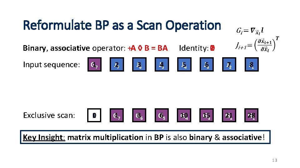
Reformulate BP as a Scan Operation Binary, associative operator: +A ◊ B = BA Identity: I 0 Input sequence: G 17 J 27 J 36 J 45 J 54 J 63 J 72 J 81 Exclusive scan: 0 I G 17 G 36 G 65 10 G 4 15 G 3 21 G 2 28 G 1 Key Insight: matrix multiplication in BP is also binary & associative! 13

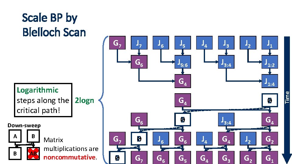
G 17 J 27 J 36 G 36 Logarithmic steps along the 2 logn critical path! A B B Matrix multiplications are AB BA noncommutative. J 54 J 5: 6 7 G 36 Down-sweep J 45 J 63 J 72 J 11 3: 4 J 81 J 15 1: 2 10 G 4 J 26 1: 4 10 G 4 I 0 J 11 3: 4 I 0 10 G 4 G 17 I 0 J 36 G 36 J 54 10 G 4 J 72 21 G 2 I 0 G 17 G 36 G 65 10 G 4 15 G 3 21 G 2 28 G 1 Time Scale BP by Blelloch Scan

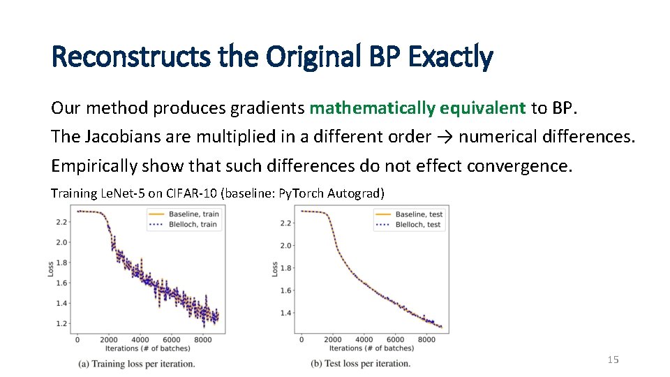
Reconstructs the Original BP Exactly Our method produces gradients mathematically equivalent to BP. The Jacobians are multiplied in a different order → numerical differences. Empirically show that such differences do not effect convergence. Training Le. Net-5 on CIFAR-10 (baseline: Py. Torch Autograd) 15

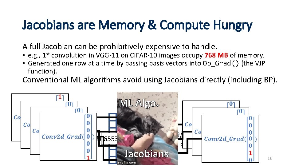
Jacobians are Memory & Compute Hungry A full Jacobian can be prohibitively expensive to handle. • e. g. , 1 st convolution in VGG-11 on CIFAR-10 images occupy 768 MB of memory. • Generated one row at a time by passing basis vectors into Op_Grad() (the VJP function). Conventional ML algorithms avoid using Jacobians directly (including BP). 3072 ML Algo. 65536 768 MB Jacobians 16

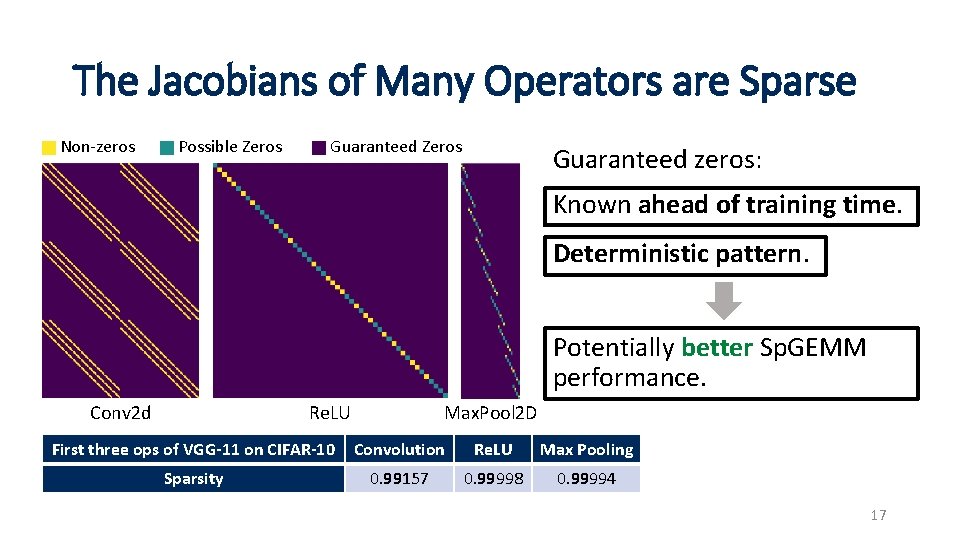
The Jacobians of Many Operators are Sparse Non-zeros Possible Zeros Guaranteed zeros: Known ahead of training time. Deterministic pattern. Potentially better Sp. GEMM performance. Conv 2 d Re. LU Max. Pool 2 D First three ops of VGG-11 on CIFAR-10 Convolution Re. LU Max Pooling Sparsity 0. 99157 0. 99998 0. 99994 17

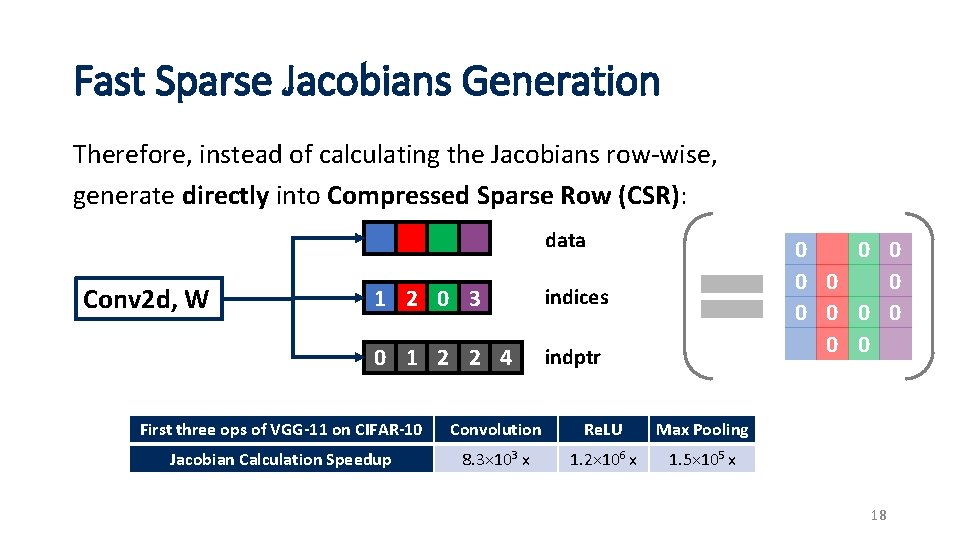
Fast Sparse Jacobians Generation Therefore, instead of calculating the Jacobians row-wise, generate directly into Compressed Sparse Row (CSR): data Conv 2 d, W 1 2 0 3 indices 0 1 2 2 4 indptr 0 0 0 First three ops of VGG-11 on CIFAR-10 Convolution Re. LU Max Pooling Jacobian Calculation Speedup 8. 3× 103 x 1. 2× 106 x 1. 5× 105 x 18

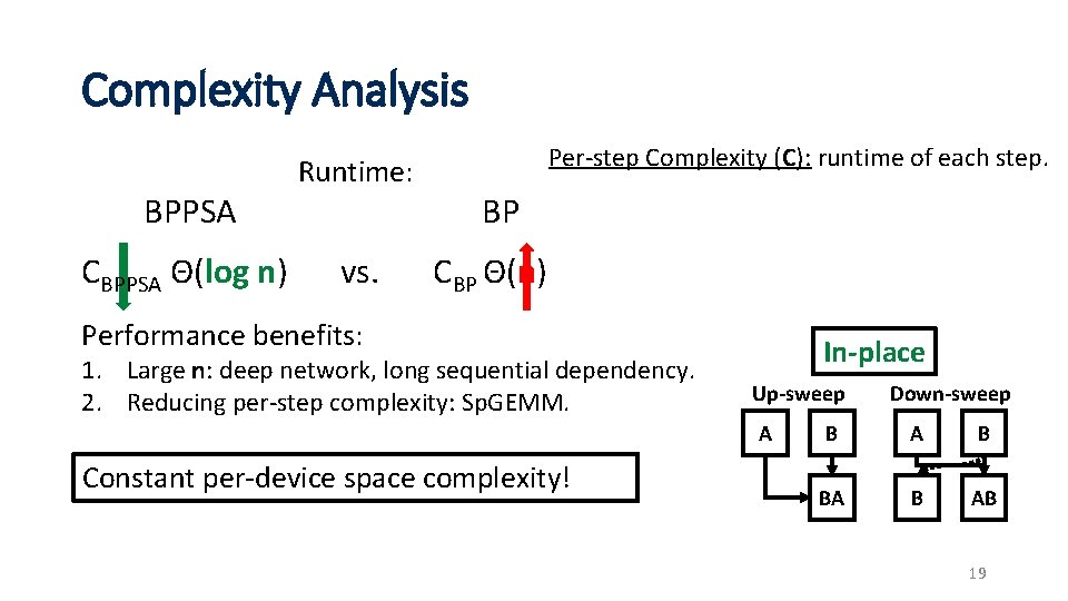
Complexity Analysis BPPSA CBPPSA Θ(log n) Runtime: vs. Per-step Complexity (C): runtime of each step. BP CBP Θ(n) Performance benefits: 1. Large n: deep network, long sequential dependency. 2. Reducing per-step complexity: Sp. GEMM. In-place Up-sweep A Constant per-device space complexity! Down-sweep B A B BA B AB 19

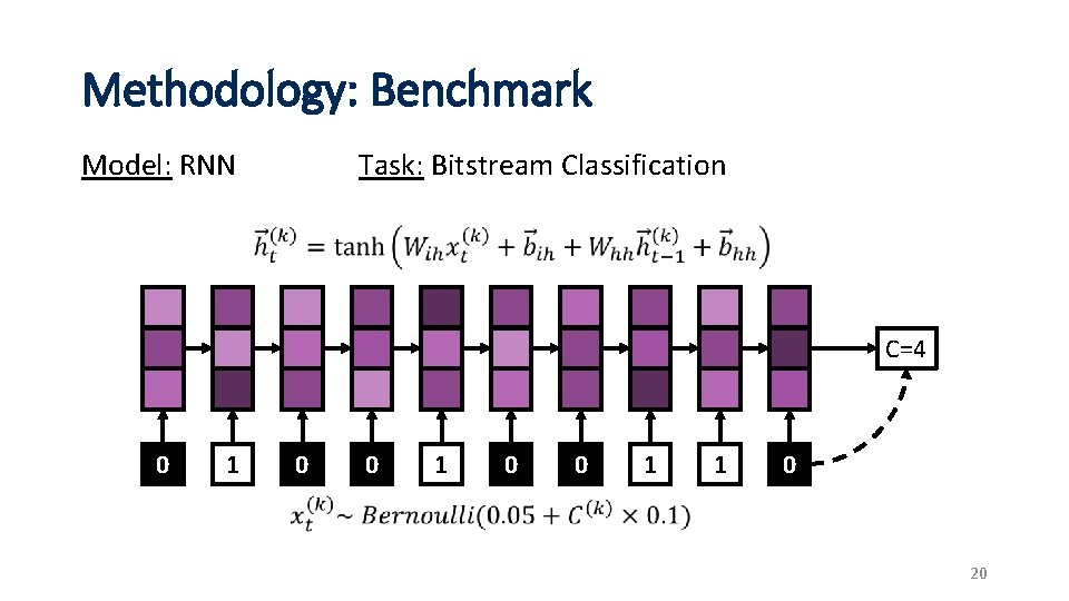
Methodology: Benchmark Task: Bitstream Classification Model: RNN V 100 C=4 0 1 0 0 1 1 0 20

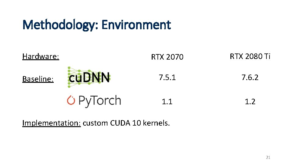
Methodology: Environment Hardware: Baseline: RTX 2070 RTX 2080 Ti 7. 5. 1 7. 6. 2 1. 1 1. 2 Implementation: custom CUDA 10 kernels. 21

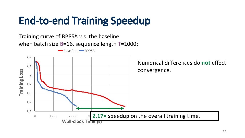
End-to-end Training Speedup Training curve of BPPSA v. s. the baseline when batch size B=16, sequence length T=1000: Baseline BPPSA 2, 4 Numerical differences do not effect convergence. Training Loss 2, 2 2 1, 8 1, 6 1, 4 1, 2 0 1000 2000 5000 2. 17× 4000 speedup on the overall training time. 3000 Wall-clock Time (s) 22

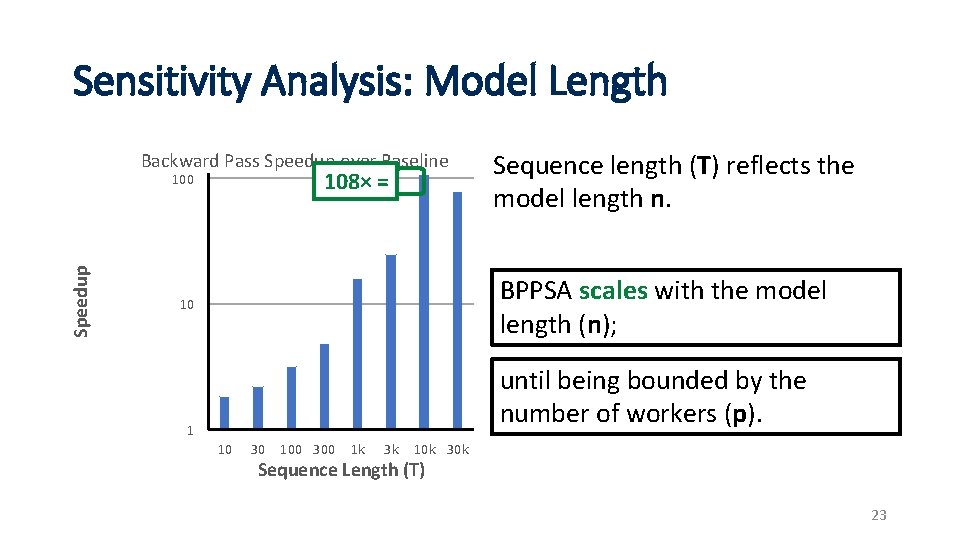
Sensitivity Analysis: Model Length Backward Pass Speedup over Baseline 108× = Speedup 100 Sequence length (T) reflects the model length n. BPPSA scales with the model length (n); 10 until being bounded by the number of workers (p). 1 10 30 100 300 1 k 3 k 10 k 30 k Sequence Length (T) 23

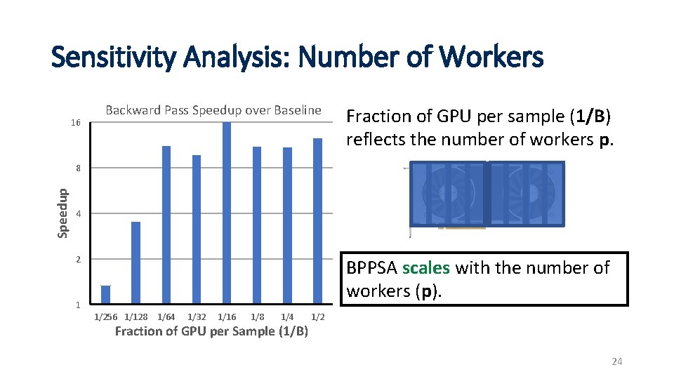
Sensitivity Analysis: Number of Workers 16 Backward Pass Speedup over Baseline Fraction of GPU per sample (1/B) reflects the number of workers p. Speedup 8 4 2 1 BPPSA scales with the number of workers (p). 1/256 1/128 1/64 1/32 1/16 1/8 1/4 Fraction of GPU per Sample (1/B) 1/2 24

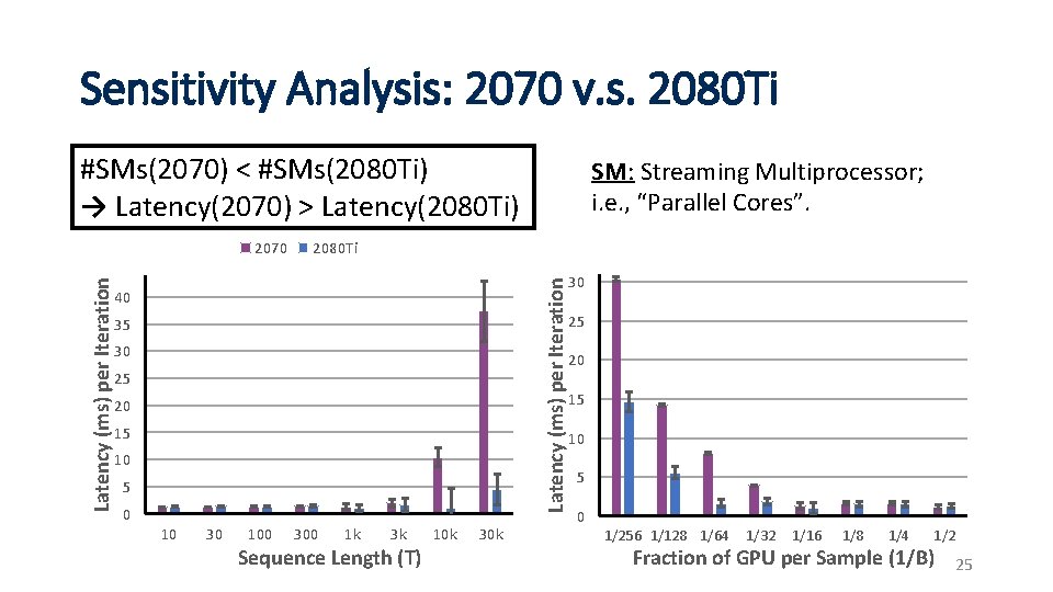
Sensitivity Analysis: 2070 v. s. 2080 Ti #SMs(2070) < #SMs(2080 Ti) → Latency(2070) > Latency(2080 Ti) 2080 Ti Latency (ms) per Iteration 2070 SM: Streaming Multiprocessor; i. e. , “Parallel Cores”. 40 35 30 25 20 15 10 5 0 10 30 100 300 1 k 3 k Sequence Length (T) 10 k 30 25 20 15 10 5 0 1/256 1/128 1/64 1/32 1/16 1/8 1/4 1/2 Fraction of GPU per Sample (1/B) 25

More Results in the Paper • End-to-end benchmarks of GRU training on IRMAS. • A more realistic version of the RNN results. • Pruned VGG-11 retraining on CIFAR-10. • Microbenchmark via FLOP measurements. • Evaluate the effectiveness of leveraging the Jacobians’ sparsity in CNNs. 26

Conclusion BP imposes a strong sequential dependency among layers during the gradient computations, limiting its scalability on parallel systems. We propose scaling Back-Propagation by Parallel Scan Algorithm (BPPSA): • Reformulate BP as a scan operation. • Scale by a customized Blelloch scan algorithm. • Leverage sparsity in the Jacobians. Key Results: Θ(log n) vs. Θ(n) steps on parallel systems. Up to 108× speedup on the backward pass (→ 2. 17× overall speedup). 27