Scalable Machine Learning Computing Summarization in a Parallel

Scalable Machine Learning Computing Summarization in a Parallel Database System Carlos Ordonez 1

Acknowledgments • Michael Stonebraker, MIT (Sci. DB) • Divsh Srivastava, Simon Urbanek: ATT Labs (R language runtime) • My Ph. D students: Yiqun Zhang, Wellington Cabrera, Huy Hoang 2

Parallel data analytics architecture • Shared-nothing, messagepassing • N nodes • Data partitioned before computation: load time • Examples: Parallel DBMSs, Hadoop HDFS, Map. Reduce, Spark

4

Example: Linear regression

Old: separate sufficient statistics, used for K-means and EM clustering, Q diagonal! 6

New: Generalizing and integrating Sufficient Statistics: Z=[1, X, Y]; full matrix! 7

Linear Algebra: Our Main Equation for Parallel/Scalable Computation

Descriptive statistics & statistical models benefiting from Gamma • • Descriptive statistics on multiple data subsets Covariance and correlation matrices Linear regression PCA EM for mixtures of Gaussians and K-means Linear Discriminant Analysis Naïve Bayesian variable selection with Gibbs sampler

Equivalent equations with projections from Gamma (descriptive, predictive) 10

2 -phase algorithm

System components and data flow

Example: R program Gamma = function(arr. Name) { strquery = paste("Dense. Gamma(", arr. Name, ")", sep="") Gamma_vertical = iquery(strquery, return=TRUE) d = max(Gamma_vertical$i) Gamma = matrix(0, nrow=d, ncol=d) k=1 for (i in 1: d) for (j in 1: d) { Gamma[i, j] = Gamma_vertical[k, 3] k = k+1 } return(Gamma) } LR = function(Gamma) { d = dim(Gamma)[1] - 2 Q = Gamma[2: (d+1), 2: (d+1)] XYT = Gamma[2: (d+1), d+2] Beta = solve(Q) %*% XYT return(Beta) }

Fundamental properties: noncommutative but distributive 15

Parallel Theoretical Guarantees of 16

Computation: Parallel array DBMS • Sci. DB: Large matrices beyond RAM size; storage by row or column not good enough • Matrices natural in statistics, machine learn. and science • Parallel shared-nothing best for big data analytics • Some similarities with HDFS+Map. Reduce • Feasible to create array operators, having matrices as input and matrix as output • Leverage R language and LAPACK 17

Array storage and processing in Sci. DB • Assuming d<<n it is natural to hash partition X by i=1. . n • Gamma computation is fully parallel maintaining local Gamma versions in RAM. • X can be read with a fully parallel scan • No need to write Gamma from RAM to disk during scan, unless fault tolerant 18

Point must fit in one chunk. Otherwise, join is needed (slow) 1 2 d 2 2 d NO! OK Coordinator 1 1 d Coordinator Worker 1 19

Dense matrix operator: O(d 2 n) 20

Sparse matrix operator: O(dn) for hyper-sparse matrix 21

Pros: Algorithm evaluation with physical array operators • Since xi fits in one chunk joins are avoided (at least 2 X I/O with hash or merge join) • Since zi*zi. T can be computed in RAM we avoid an aggregation which would require sort • No need to store X twice: X, XT: half I/O, half RAM • No need to transpose X or Z, costly reorganization even in RAM • Operator works in C++ compiled code: fast; vector accessed once; direct assignment (bypass C++ functions calls) 22

Optimization: GPU • The C++ operator code is annotated with Open. ACC directives to work with GPU • The CPU only does the I/O part in the current implementation. • Data is transferred from host memory to device (GPU) memory • The vector outer products are evaluated and aggregated on GPU, the result is then transferred back.

System issues and limitations • Gamma not efficiently computable in AQL/AFL: oper. required • Arrays of tuples in Sci. DB are more general, but cumbersome for matrix manipulation: arrays of single attribute (double) • Points must be stored completely inside a chunk: wide rectangular chunks: may not be I/O optimal • Slow: Arrays must be pre-processed to Sci. DB load format, loaded to 1 D array and re-dimensioned=>optimize load. • Multiple Sci. DB instances per node improve I/O speed: interleaving CPU • Larger chunks are better: 8 MB, especially for dense matrices; avoid shuffling; avoid joins • Dense (alpha) and sparse (beta) versions 24

Benchmark time comparison • Compare with R, which calls LAPACK • Parallel processing: Spark vs R+Sci. DB • Acceleration with GPU (~1500 cores) 25

Comparing: R alone with R+Sci. DB 26

27

Why is Gamma faster than Sci. DB+LAPACK? Gamma operator Gamma d op 100 200 400 800 1600 3. 5 10. 9 38. 8 145. 0 599. 8 Scan mem alloc 0. 7 1. 0 2. 2 4. 6 11. 4 0. 1 0. 1 CPU merge 2. 2 8. 6 33. 9 134. 7 575. 5 Sci. DB and LAPACK (crossprod() call in Sci. DB) transpos TOTAL subarray 1 repart 1 subarray 2 e 77. 3 163. 0 373. 1 1497. 3 * 0. 1 * 0. 3 0. 2 0. 3 0. 1 * 41. 7 84. 9 172. 6 553. 6 * 0. 1 0. 5 0. 8 * 0. 0 0. 1 0. 4 1. 0 repart 2 25. 9 55. 7 120. 6 537. 6 * build 0 s 0. 0 0. 3 0. 5 * gemm 8. 0 17. 2 39. 4 169. 8 * Sca. LAPACK MKL 0. 8 1. 8 5. 4 21. 2 * 0. 2 0. 6 2. 1 8. 1 33. 4 28

Can Gamma operator beat LAPACK? Gamma versus Open BLAS LAPACK (90% performance of MKL) Gamma: scan, sparse/dense 2 threads; disk+RAM+CPU LAPACK: Open BLAS~=MKL; 2 threads; RAM+CPU d=100 LAPACK d=200 LAPACK d=400 dens spars ndensity e e Op BLAS dense sparse LAPACK d=800 Op BLAS 2 dense LAPACK sparse Open BLAS 100 k 0. 1% 3. 3 0. 1 0. 4 11. 3 0. 1 1. 0 38. 9 0. 2 3. 1 145. 0 0. 6 10. 7 100 k 1. 0% 3. 3 0. 1 0. 4 11. 3 0. 2 1. 0 38. 9 0. 4 3. 1 145. 0 10. 7 100 k 10. 0% 3. 3 0. 5 0. 4 11. 3 0. 9 1. 0 38. 9 2. 2 3. 1 145. 0 6. 2 10. 7 100 k 1 M 1 M 100. 0% 0. 1% 1. 0% 100. 0% 3. 3 4. 5 31. 1 0. 2 31. 1 0. 5 31. 1 4. 0 31. 1 44. 0 0. 4 3. 8 11. 3 15. 4 103. 5 0. 2 103. 5 1. 1 103. 5 7. 0 103. 5 148. 8 1. 0 10. 0 38. 9 316. 5 55. 9 0. 4 3. 8 16. 3 542. 3 3. 1 423. 2 145. 0 1475. 7 201. 0 0. 9 fail 4. 0 fail 46. 4 fail 2159. 6 fail 10. 7 29

Computing Γ amma on local server

Alternative parallel DBMS Columnar vs. array for sparse matrices

Cloud: Comparison with Apache Spark in large parallel cluster •

Linear Regression (prototype model) Parallel Array DBMS vs Spark

Gamma matrix: as Gramian product Parallel Array DBMS vs Spark

Running in the cloud, 100 nodes

Further optimization: GPU (1536 cores, 4 GB GPU mem) Transfer Summarize Transfer GPU

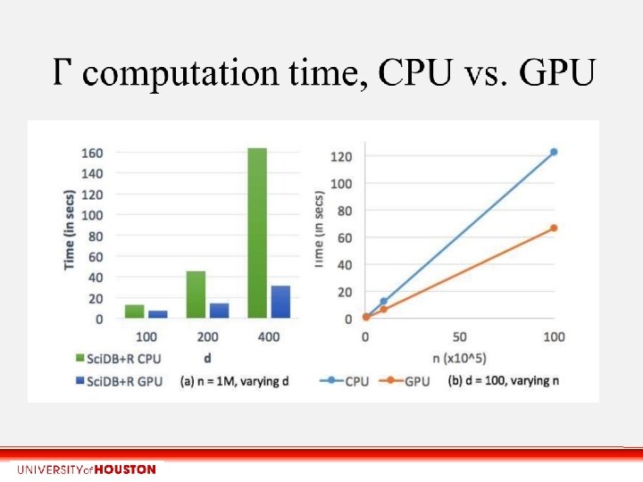
Time saved by summarizing on GPU n = 1 M d = 400

Conclusions • One pass summarization matrix operator: highly parallel, scalable, compatible with any parallel system • Optimization of Gramian matrix multiplication: sum (aggregation) of vector outer products • Dense and sparse matrix versions required • Reduces methods to two phases: 1: Summarization, 2: Computing model parameters. • Requires arrays, but can work with SQL tables or Map. Reduce files or Spark’s RDD data sets • Gamma matrix must fit in RAM, but n unlimited 39

Future work • Exploit Gamma in other models like logistic regression, probit Bayesian models, EM mixtures of Gaussians, Factor Analysis, HMMs • Online model learning (streams) • Higher-order expected moments, co-variates • Analytics in data science shifting to Python • HPC: can Gamma beat Sca. LAPACK with sparse matrices? 40