SC 968 Panel data methods for sociologists Lecture

SC 968 Panel data methods for sociologists Lecture 2, part 1 Introducing panel data

Overview ¢ Panel data l l ¢ What it is How to get to know the data Change over time l l Tabulating Calculating transition probabilities

What is panel data? ¢ A data set containing observations on multiple phenomena observed at a single point in time is called cross-sectional data ¢ A data set containing observations on a single phenomenon observed over multiple time periods is called time series data ¢ Observations on multiple phenomena over multiple time periods are panel data ¢ Cross sectional and time series data are one- dimensional, panel data are two-dimensional l Panel data can be used to answer both longitudinal and crosssectional questions!

Using panel data in Stata ¢ Data on n cases, over t time periods, giving a total of n × t observations ¢ One record per observation i. e. long format ¢ Stata tools for analyzing panel data begin with the prefix xt ¢ First need to tell Stata that you have panel data using xtset

Complete and incomplete person-wave data

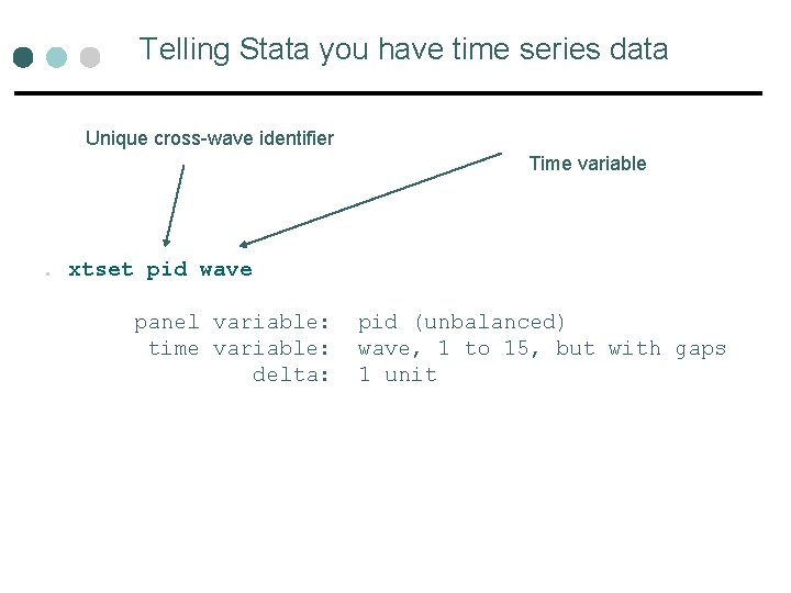
Telling Stata you have time series data Unique cross-wave identifier Time variable . xtset pid wave panel variable: time variable: delta: pid (unbalanced) wave, 1 to 15, but with gaps 1 unit

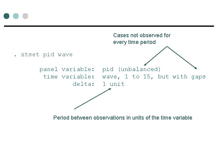
Cases not observed for every time period . xtset pid wave panel variable: time variable: delta: pid (unbalanced) wave, 1 to 15, but with gaps 1 unit Period between observations in units of the time variable

Describing the patterns in panel data

Examining change over two waves

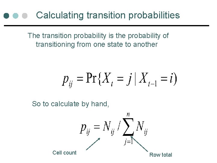
Calculating transition probabilities The transition probability is the probability of transitioning from one state to another So to calculate by hand, Cell count Row total

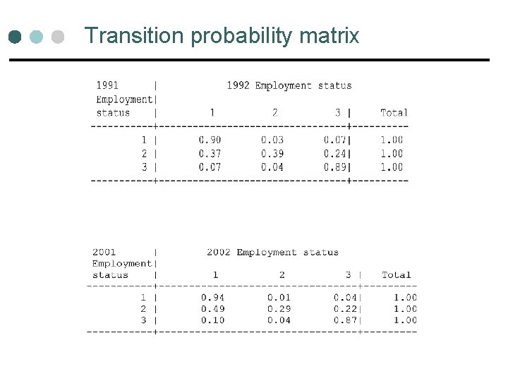
Transition probability matrix

Transition probability matrices in Stata Mean transition probabilities for all waves t to t+1 when you leave out the “if” statement

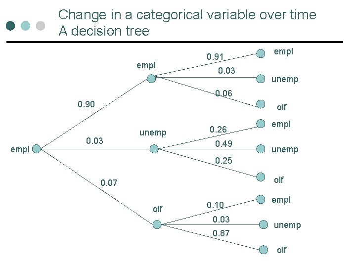
Change in a categorical variable over time A decision tree empl 0. 91 0. 03 empl unemp 0. 06 0. 90 empl olf 0. 03 unemp 0. 26 0. 49 empl unemp 0. 25 olf 0. 07 olf 0. 10 0. 03 0. 87 empl unemp olf

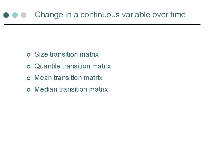
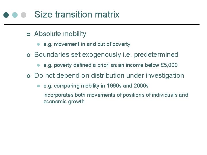
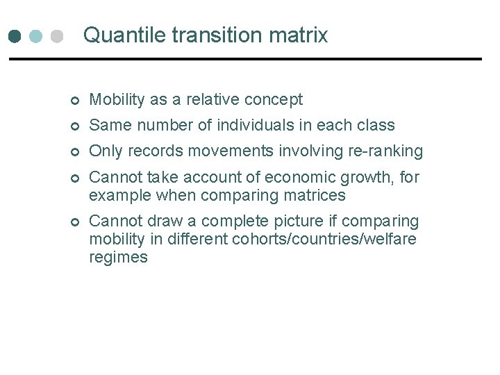
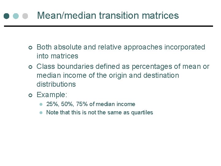
Change in a continuous variable over time ¢ Size transition matrix ¢ Quantile transition matrix ¢ Mean transition matrix ¢ Median transition matrix

Size transition matrix ¢ Absolute mobility l ¢ Boundaries set exogenously i. e. predetermined l ¢ e. g. movement in and out of poverty e. g. poverty defined a priori as an income below £ 5, 000 Do not depend on distribution under investigation l e. g. comparing mobility in 1990 s and 2000 s incorporates both movements of positions of individuals and economic growth

Quantile transition matrix ¢ Mobility as a relative concept ¢ Same number of individuals in each class ¢ Only records movements involving re-ranking ¢ Cannot take account of economic growth, for example when comparing matrices ¢ Cannot draw a complete picture if comparing mobility in different cohorts/countries/welfare regimes

Mean/median transition matrices ¢ ¢ ¢ Both absolute and relative approaches incorporated into matrices Class boundaries defined as percentages of mean or median income of the origin and destination distributions Example: l l 25%, 50%, 75% of median income Note that this is not the same as quartiles

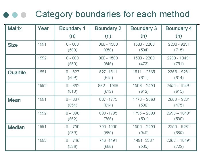
Example: income 1991 -1992

Category boundaries for each method Matrix Year Boundary 1 (n) Boundary 2 (n) Boundary 3 (n) Boundary 4 (n) Size 1991 0 - 800 (580) 800 - 1500 (650) 1500 - 2200 (504) 2200 - 9231 (715) 1992 0 - 800 (580) 800 - 1500 (645) 1500 - 2200 (473) 2200 - 10491 (751) 1991 0 – 827 (609) 827 -1511 (615) 1511 – 2365 (611) 2365 – 9231 (614) 1992 0 – 862 (610) 862 – 1508 (612) 1508 – 2450 (612) 2450 – 10491 (615) 1991 0 – 887 (654) 887 -1773 (814) 1773 – 2660 (506) 2660 – 9231 (475) 1992 0 – 898 (652) 898 -1795 (766) 1795 – 2693 (501) 2693 – 10491 (530) 1991 0 – 750 (539) 750 -1500 (685) 1500 – 2250 (540) 2250 – 9231 (685) 1992 0 – 746 (536) 746 -1491 (686) 1491 -2237 (505) 2262 – 10491 (722) Quartile Mean Median

Warning! ¢ Measurement error l Causes an over-estimation of mobility l If mother’s and baby’s weight are reported to nearest half pound can affect which band the observations falls in l A respondent may describe their marital status as separated in year 1 and single in year 2

Finally…. . ¢ ¢ Greater challenges to understanding and checking panel data Transition matrices a good way to summarise mobility patterns Different methods of constructing matrices lead to distinct interpretations May need to take account of measurement error when modelling change

SC 968 Panel data methods for sociologists Lecture 2, part 2 Concepts for panel data analysis

Overview ¢ ¢ ¢ Types of questions, types of variables: time-invariant, time-varying and trend Between- and within-individual variation Concept of individual heterogeneity From OLS to models that allow causal interpretations: fixed effects and random effects models The basics of these models’ implementation in Stata

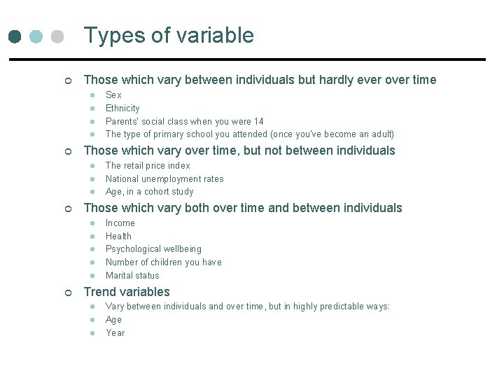
Types of variable ¢ Those which vary between individuals but hardly ever over time l l ¢ Those which vary over time, but not between individuals l l l ¢ The retail price index National unemployment rates Age, in a cohort study Those which vary both over time and between individuals l l l ¢ Sex Ethnicity Parents’ social class when you were 14 The type of primary school you attended (once you’ve become an adult) Income Health Psychological wellbeing Number of children you have Marital status Trend variables l l l Vary between individuals and over time, but in highly predictable ways: Age Year

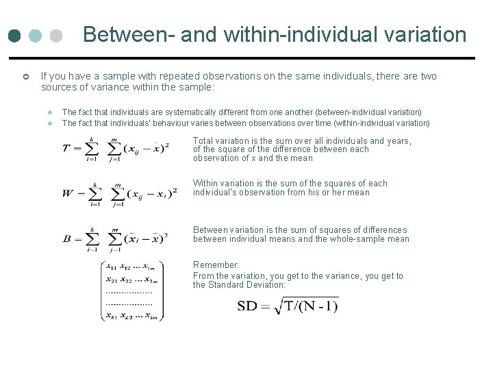
Between- and within-individual variation ¢ If you have a sample with repeated observations on the same individuals, there are two sources of variance within the sample: l l The fact that individuals are systematically different from one another (between-individual variation) The fact that individuals’ behaviour varies between observations over time (within-individual variation) Total variation is the sum over all individuals and years, of the square of the difference between each observation of x and the mean Within variation is the sum of the squares of each individual’s observation from his or her mean Between variation is the sum of squares of differences between individual means and the whole-sample mean Remember: From the variation, you get to the variance, you get to the Standard Deviation:

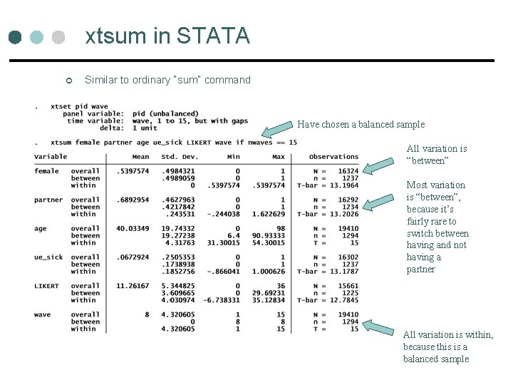
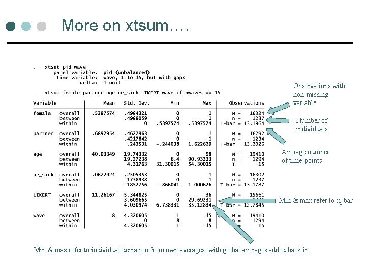
xtsum in STATA ¢ Similar to ordinary “sum” command Have chosen a balanced sample All variation is “between” Most variation is “between”, because it’s fairly rare to switch between having and not having a partner All variation is within, because this is a balanced sample

More on xtsum…. Observations with non-missing variable Number of individuals Average number of time-points Min & max refer to xi-bar Min & max refer to individual deviation from own averages, with global averages added back in.

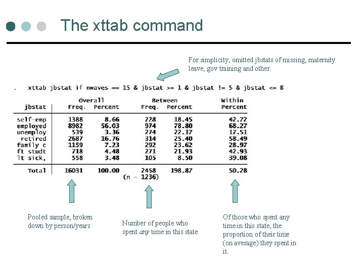
The xttab command For simplicity, omitted jbstats of missing, maternity leave, gov training and other. Pooled sample, broken down by person/years Number of people who spent any time in this state Of those who spent any time in this state, the proportion of their time (on average) they spent in it.

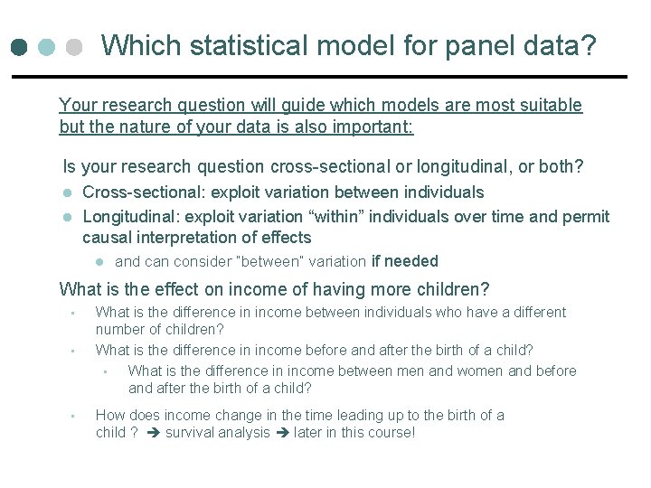
Which statistical model for panel data? Your research question will guide which models are most suitable but the nature of your data is also important: Is your research question cross-sectional or longitudinal, or both? l l Cross-sectional: exploit variation between individuals Longitudinal: exploit variation “within” individuals over time and permit causal interpretation of effects l and can consider “between” variation if needed What is the effect on income of having more children? • • • What is the difference in income between individuals who have a different number of children? What is the difference in income before and after the birth of a child? • What is the difference in income between men and women and before and after the birth of a child? How does income change in the time leading up to the birth of a child ? survival analysis later in this course!

Longitudinal analysis is concerned with modelling individual heterogeneity ¢ ¢ A very simple concept: people are different! In social science, when we talk about heterogeneity, we are really talking about unobservable (or unobserved) heterogeneity: Observed heterogeneity: differences in education levels, or parental background, or anything else that we can measure and control for in regressions Unobserved heterogeneity: anything which is fundamentally unmeasurable, or which is rather poorly measured, or which does not happen to be measured in the particular data set we are using. ¢ With panel data we can do something about unobserved heterogeneity as we can differentiate between person-level unobserved x that are identical over time and those that vary over time!

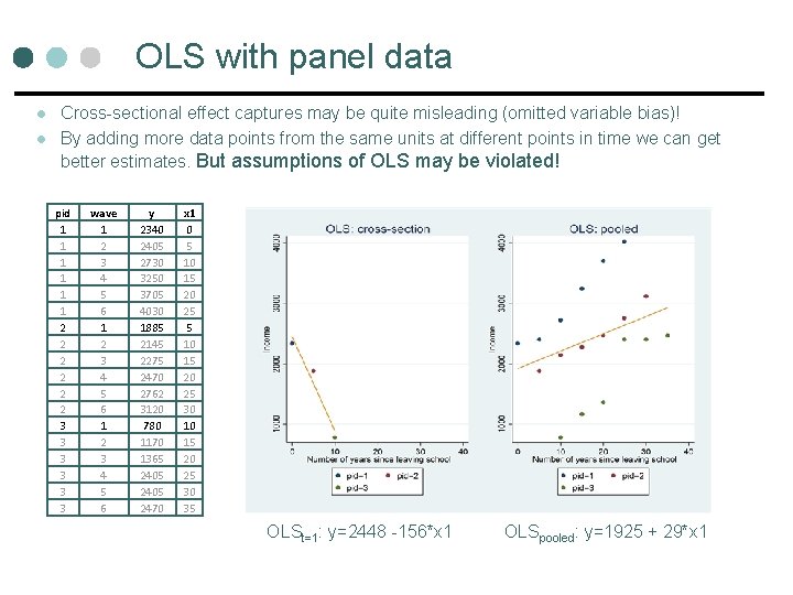
OLS with panel data l l Cross-sectional effect captures may be quite misleading (omitted variable bias)! By adding more data points from the same units at different points in time we can get better estimates. But assumptions of OLS may be violated! pid 1 1 1 2 2 2 3 3 3 wave 1 2 3 4 5 6 y 2340 2405 2730 3250 3705 4030 1885 2145 2275 2470 2762 3120 780 1170 1365 2405 2470 x 1 0 5 10 15 20 25 30 35 OLSt=1: y=2448 -156*x 1 OLSpooled: y=1925 + 29*x 1

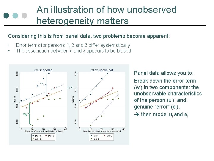
An illustration of how unobserved heterogeneity matters Considering this is from panel data, two problems become apparent: • • Error terms for persons 1, 2 and 3 differ systematically The association between x and y appears to be biased w 1 w 3 u 1 ? Panel data allows you to: Break down the error term (wi) in two components: the unobservable characteristics of the person (ui), and genuine “error” (ei). then model ui and ei

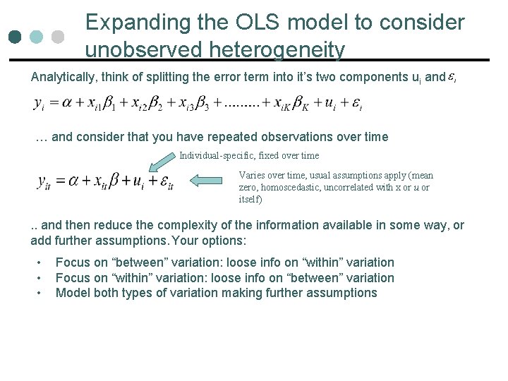
Expanding the OLS model to consider unobserved heterogeneity Analytically, think of splitting the error term into it’s two components ui and … and consider that you have repeated observations over time Individual-specific, fixed over time Varies over time, usual assumptions apply (mean zero, homoscedastic, uncorrelated with x or u or itself) . . and then reduce the complexity of the information available in some way, or add further assumptions. Your options: • • • Focus on “between” variation: loose info on “within” variation Focus on “within” variation: loose info on “between” variation Model both types of variation making further assumptions

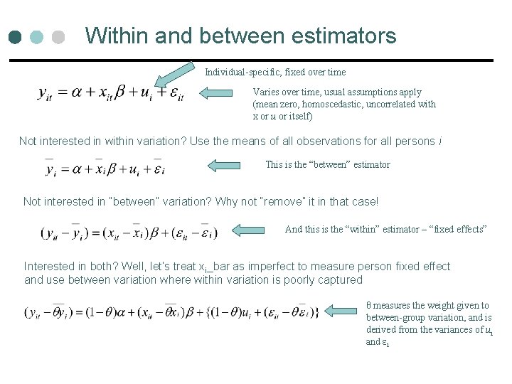
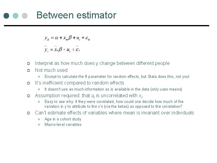
Within and between estimators Individual-specific, fixed over time Varies over time, usual assumptions apply (mean zero, homoscedastic, uncorrelated with x or u or itself) Not interested in within variation? Use the means of all observations for all persons i This is the “between” estimator Not interested in “between” variation? Why not “remove” it in that case! And this is the “within” estimator – “fixed effects” Interested in both? Well, let’s treat xi_bar as imperfect to measure person fixed effect and use between variation where within variation is poorly captured θ measures the weight given to between-group variation, and is derived from the variances of ui and εi

Between estimator ¢ ¢ Interpret as how much does y change between different people Not much used l ¢ It’s inefficient compared to random effects l ¢ It doesn’t use as much information as is available in the data (only uses means) Assumption required: that ui is uncorrelated with xi l ¢ Except to calculate the θ parameter for random effects, but Stata does this, not you! Easy to see why: if they were correlated, how could one decide how much of the variation in y to attribute to the x’s (via the betas) as opposed to the correlation? Can’t estimate effects of variables where mean is invariant over individuals l l Age in a cohort study Macro-level variables

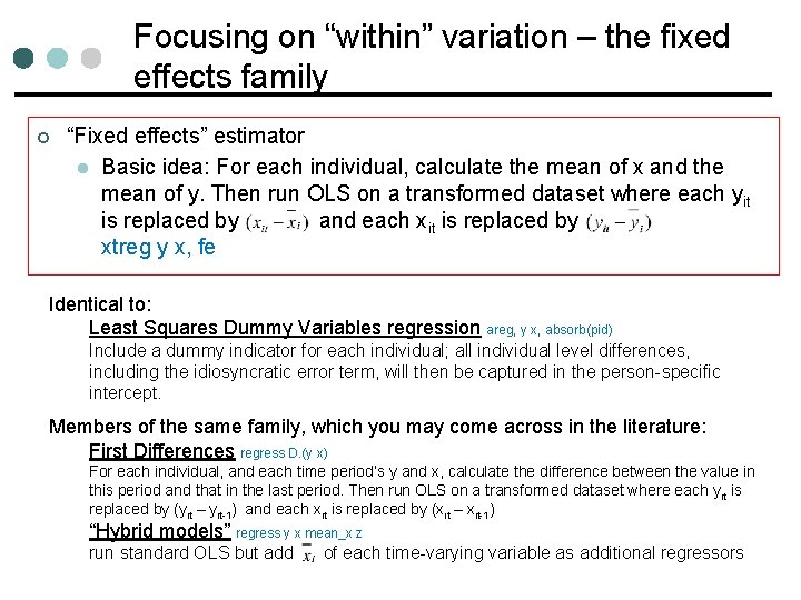
Focusing on “within” variation – the fixed effects family ¢ “Fixed effects” estimator l Basic idea: For each individual, calculate the mean of x and the mean of y. Then run OLS on a transformed dataset where each yit is replaced by and each xit is replaced by xtreg y x, fe Identical to: Least Squares Dummy Variables regression areg, y x, absorb(pid) Include a dummy indicator for each individual; all individual level differences, including the idiosyncratic error term, will then be captured in the person-specific intercept. Members of the same family, which you may come across in the literature: First Differences regress D. (y x) For each individual, and each time period’s y and x, calculate the difference between the value in this period and that in the last period. Then run OLS on a transformed dataset where each y it is replaced by (yit – yit-1) and each xit is replaced by (xit – xit-1) “Hybrid models” regress y x mean_x z run standard OLS but add of each time-varying variable as additional regressors

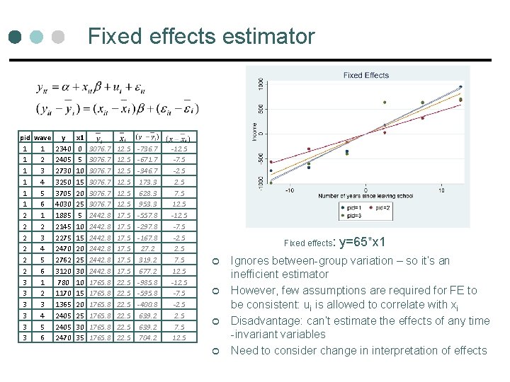
Fixed effects estimator pid wave y x 1 1 1 2340 0 3076. 7 12. 5 -736. 7 1 2 2405 5 3076. 7 12. 5 -671. 7 1 3 2730 10 3076. 7 12. 5 -346. 7 1 4 3250 15 3076. 7 12. 5 173. 3 1 5 3705 20 3076. 7 12. 5 628. 3 1 6 4030 25 3076. 7 12. 5 953. 3 2 1 1885 5 2442. 8 17. 5 -557. 8 2 2 2145 10 2442. 8 17. 5 -297. 8 2 3 2275 15 2442. 8 17. 5 -167. 8 2 4 2470 20 2442. 8 17. 5 27. 2 2 5 2762 25 2442. 8 17. 5 319. 2 2 6 3120 30 2442. 8 17. 5 677. 2 3 1 780 10 1765. 8 22. 5 -985. 8 3 2 1170 15 1765. 8 22. 5 -595. 8 3 3 1365 20 1765. 8 22. 5 -400. 8 3 4 2405 25 1765. 8 22. 5 639. 2 3 5 2405 30 1765. 8 22. 5 639. 2 3 6 2470 35 1765. 8 22. 5 704. 2 -12. 5 -7. 5 -2. 5 7. 5 12. 5 -12. 5 -7. 5 -2. 5 7. 5 12. 5 Fixed effects: ¢ ¢ y=65*x 1 Ignores between-group variation – so it’s an inefficient estimator However, few assumptions are required for FE to be consistent: ui is allowed to correlate with xi Disadvantage: can’t estimate the effects of any time -invariant variables Need to consider change in interpretation of effects

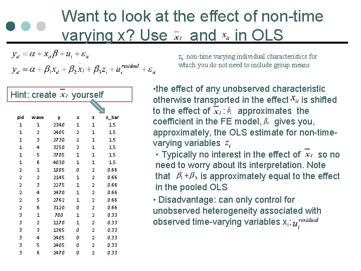
Want to look at the effect of non-time varying x? Use and in OLS zi: non-time varying individual characteristics for which you do not need to include group means Hint: create pid 1 1 1 2 2 2 3 3 3 wave 1 2 3 4 5 6 y 2340 2405 2730 3250 3705 4030 1885 2145 2275 2470 2762 3120 780 1170 1365 2405 2470 yourself x 1 2 2 2 1 1 0 0 z 1 1 1 2 2 2 x_bar 1. 5 1. 5 0. 66 0. 33 • the effect of any unobserved characteristic otherwise transported in the effect is shifted to the effect of : approximates the coefficient in the FE model, gives you, approximately, the OLS estimate for non-timevarying variables • Typically no interest in the effect of so no need to worry about its interpretation. Note that is approximately equal to the effect in the pooled OLS • Disadvantage: can only control for unobserved heterogeneity associated with observed time-varying variables xi;

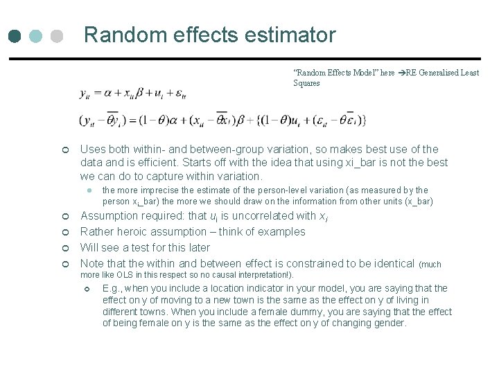
Random effects estimator “Random Effects Model” here RE Generalised Least Squares ¢ Uses both within- and between-group variation, so makes best use of the data and is efficient. Starts off with the idea that using xi_bar is not the best we can do to capture within variation. l ¢ ¢ the more imprecise the estimate of the person-level variation (as measured by the person xi_bar) the more we should draw on the information from other units (x_bar) Assumption required: that ui is uncorrelated with xi Rather heroic assumption – think of examples Will see a test for this later Note that the within and between effect is constrained to be identical (much more like OLS in this respect so no causal interpretation!). ¢ E. g. , when you include a location indicator in your model, you are saying that the effect on y of moving to a new town is the same as the effect on y of living in different towns. When you include a female dummy, you are saying that the effect of being female on y is the same as the effect on y of changing gender.

Estimating fixed effects in STATA “R-square-like” statistic Peaks at age 48 “u” and “e” are the two parts of the error term Talk about xtmixed

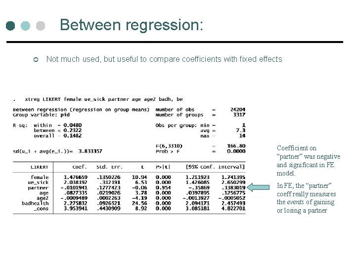
Between regression: ¢ Not much used, but useful to compare coefficients with fixed effects Coefficient on “partner” was negative and significant in FE model. In FE, the “partner” coeff really measures the events of gaining or losing a partner

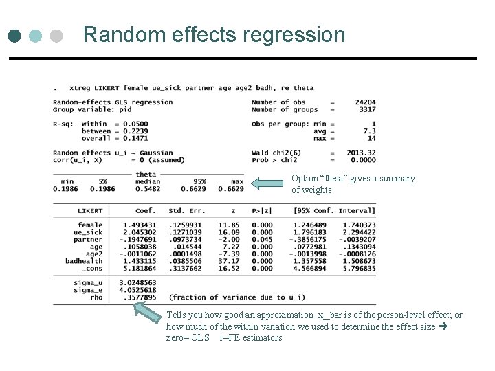
Random effects regression Option “theta” gives a summary of weights Tells you how good an approximation xi_bar is of the person-level effect; or how much of the within variation we used to determine the effect size zero= OLS 1=FE estimators

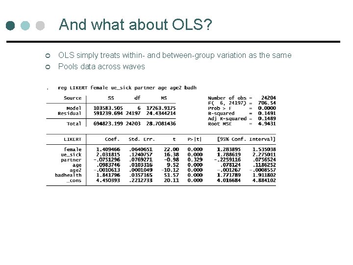
And what about OLS? ¢ ¢ OLS simply treats within- and between-group variation as the same Pools data across waves

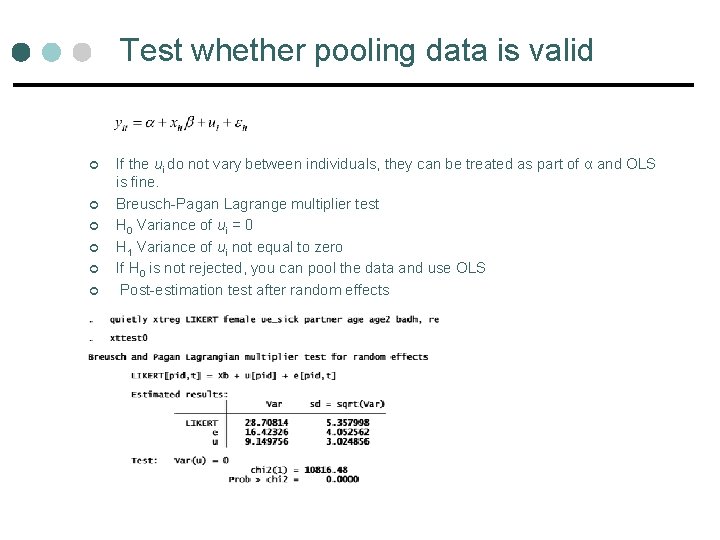
Test whether pooling data is valid ¢ ¢ ¢ If the ui do not vary between individuals, they can be treated as part of α and OLS is fine. Breusch-Pagan Lagrange multiplier test H 0 Variance of ui = 0 H 1 Variance of ui not equal to zero If H 0 is not rejected, you can pool the data and use OLS Post-estimation test after random effects

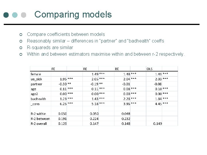
Comparing models ¢ ¢ Compare coefficients between models Reasonably similar – differences in “partner” and “badhealth” coeffs R-squareds are similar Within and between estimators maximise within and between r-2 respectively.