Saving Contents to Files in Scilab pwd it

Saving Contents to Files in Scilab pwd – it will print the current working directory of scilab (when you start scilab, the default directory is C: Program Files (x 86)scilab-5. 2. 2 ls - list all the files in the current working directory cd or chdir – these commands will change the current working directory. e. g. if you want to change current directory to scilab folder (directory) in D drive then you have to write as cd D: scilab diary – Saves the entire content of the scilab work space to one file. e. g. diary (‘content. txt’) will save the entire content of the scilab work space to content. txt.

When enter the command diary(‘content. txt’), you will be prompted as ans = 1 Then you may type whatever commands you want to execute. After completing the current work, we need to close the directory by using the command diary(0). You will now find that the file content. txt is saved in the current working directory. In place of content. txt, you may choose any other file name.

Functions with Scilab To obtain a simple integral over a sine function over the range 0 to , -->x 0=0; x 1=%pi; //range of x is from x=x 0 to x= x 1 -->X=integrate ('sin(x)', 'x', x 0, x 1)//X is the value of the definite integral Here sin(x) is our function. We can integrate any other function in the limiting range x 0 to x 1. You can define a function by using the following commands. Suppose dy/dt=y^2 -y sin(t)+cos(t), y(0)=0 is the differential equation that we need to solve. //to solve a ode(ordinary differential equation)

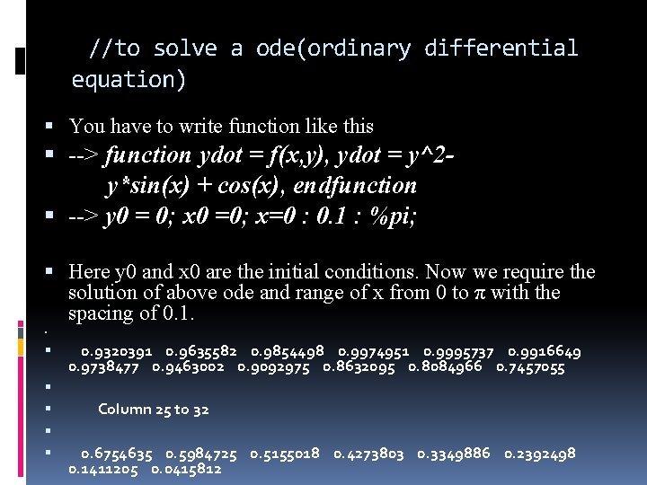
//to solve a ode(ordinary differential equation) You have to write function like this --> function ydot = f(x, y), ydot = y^2 y*sin(x) + cos(x), endfunction --> y 0 = 0; x 0 =0; x=0 : 0. 1 : %pi; Here y 0 and x 0 are the initial conditions. Now we require the solution of above ode and range of x from 0 to π with the spacing of 0. 1. 0. 9320391 0. 9635582 0. 9854498 0. 9974951 0. 9995737 0. 9916649 0. 9738477 0. 9463002 0. 9092975 0. 8632095 0. 8084966 0. 7457055 Column 25 to 32 0. 6754635 0. 5984725 0. 5155018 0. 4273803 0. 3349886 0. 2392498 0. 1411205 0. 0415812

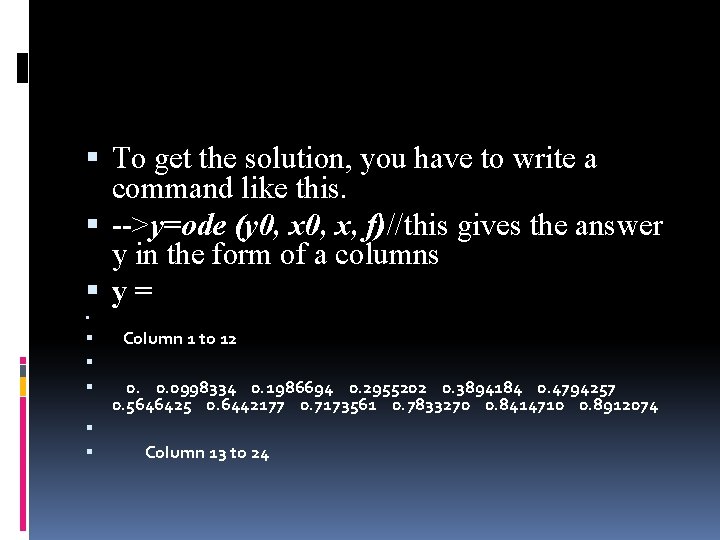
To get the solution, you have to write a command like this. -->y=ode (y 0, x, f)//this gives the answer y in the form of a columns y= Column 1 to 12 0. 0. 0998334 0. 1986694 0. 2955202 0. 3894184 0. 4794257 0. 5646425 0. 6442177 0. 7173561 0. 7833270 0. 8414710 0. 8912074 Column 13 to 24

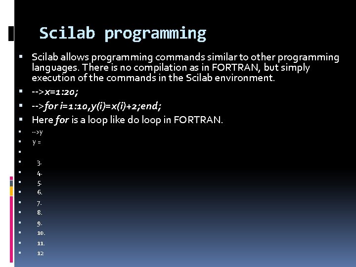
Scilab programming Scilab allows programming commands similar to other programming languages. There is no compilation as in FORTRAN, but simply execution of the commands in the Scilab environment. -->x=1: 20; -->for i=1: 10, y(i)=x(i)+2; end; Here for is a loop like do loop in FORTRAN. -->y y= 3. 4. 5. 6. 7. 8. 9. 10. 11. 12

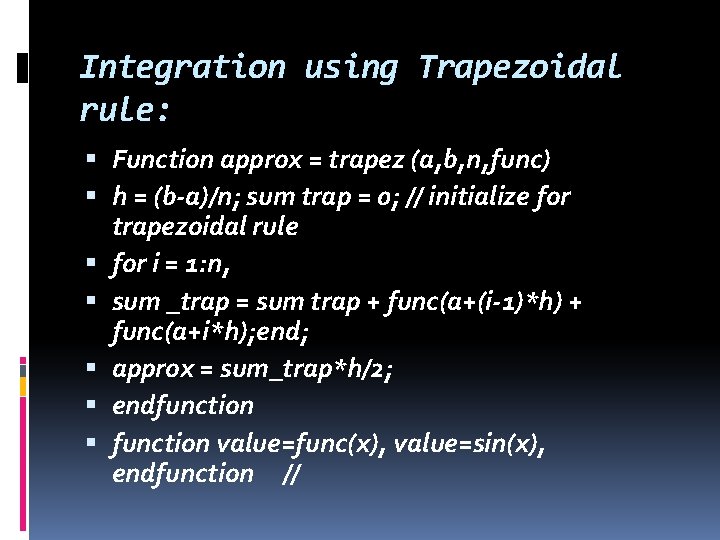
Integration using Trapezoidal rule: Function approx = trapez (a, b, n, func) h = (b-a)/n; sum trap = 0; // initialize for trapezoidal rule for i = 1: n, sum _trap = sum trap + func(a+(i-1)*h) + func(a+i*h); end; approx = sum_trap*h/2; endfunction value=func(x), value=sin(x), endfunction //

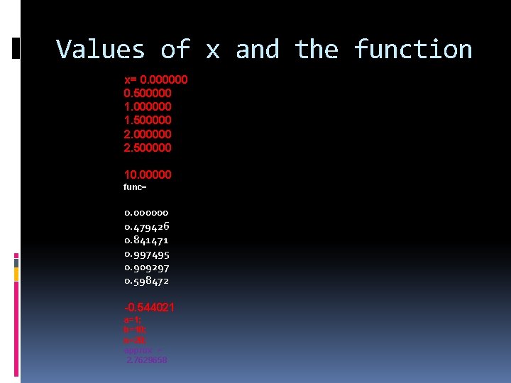
Values of x and the function x= 0. 000000 0. 500000 1. 000000 1. 500000 2. 000000 2. 500000 10. 00000 func= 0. 000000 0. 479426 0. 841471 0. 997495 0. 909297 0. 598472 -0. 544021 a=1; b=10; n=20; approx = 2. 7629658

Graphs/Plots To draw a plot for x vs y the command is plot(x, y). In Scilab, there are two types of plots. You can invoke them by using following commands. plot 2 d () plot 3 d () Now let us plot for function (2) given above. Plot(x, y) gives a 2 d plot. A typical plot will look like the on the next slide. For more details, Use the command, help plot 2 d

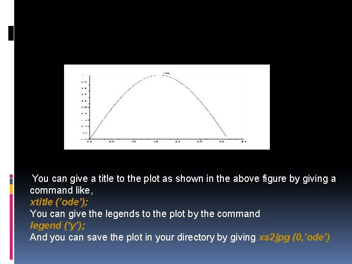
You can give a title to the plot as shown in the above figure by giving a command like, xtitle (’ode’); You can give the legends to the plot by the command legend (‘y’); And you can save the plot in your directory by giving xs 2 jpg (0, ’ode’)

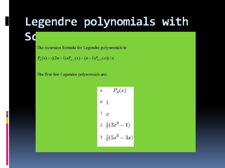
Legendre polynomials with Scilab

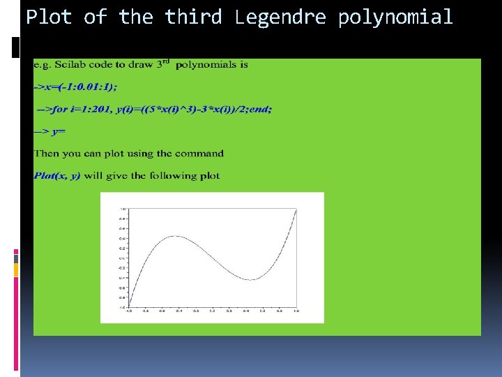
Plot of the third Legendre polynomial

Editor command in scilab We can write all commands in one page using the command called editor command. When you type editor on Scilab screen, a new window will appear where you can write all the commands and going to execute later. To execute the editor file, you have to write exec filename. sce. e. g. , Using this command, you can plot all the above 10 Legendre polynomials at once. You have to write Legendre polynomials as follows. .

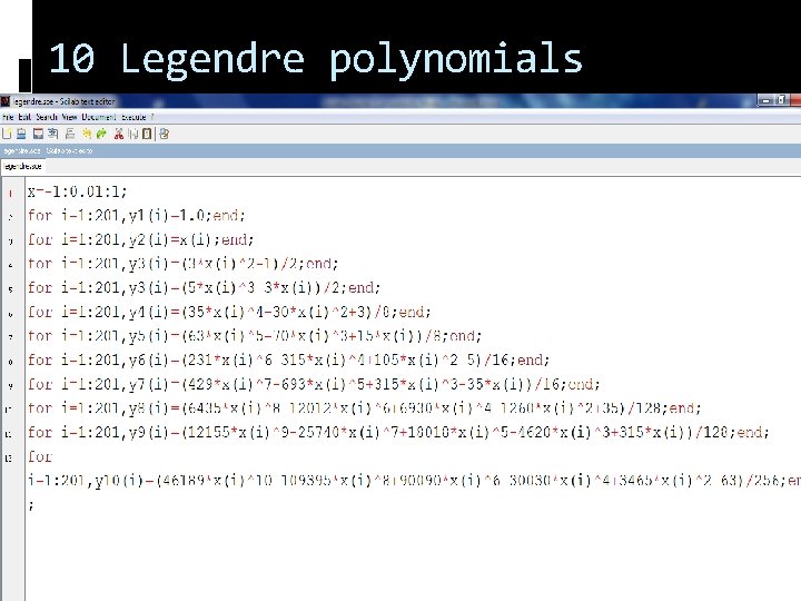
10 Legendre polynomials

Plotting 10 Legendre polynomials You have to save the file with legendre. sce file extension. And call back by the command exec legendre. sce and then you can plot using the command, plot 2 d(x, [y 1 y 2 y 3 y 4 y 5 y 6 y 7 y 8 y 9 y 10]);