SATS Transportation Systems Analysis Overview Virginia SATS Alliance

SATS Transportation Systems Analysis Overview Virginia SATS Alliance TSAA Group Meeting October 29 -30, 2002

Task Objectives • Quantify current U. S. National travel patterns as a prelude to model SATS as a feasible transportation system (the baseline for this analysis is the year 2000 ) • Develop a suitable framework and algorithms to study SATS as a feasible mode of transportation • Relate the effect of four SATS technical capabilities and how they would contribute to make SATS a feasible mode of transportation

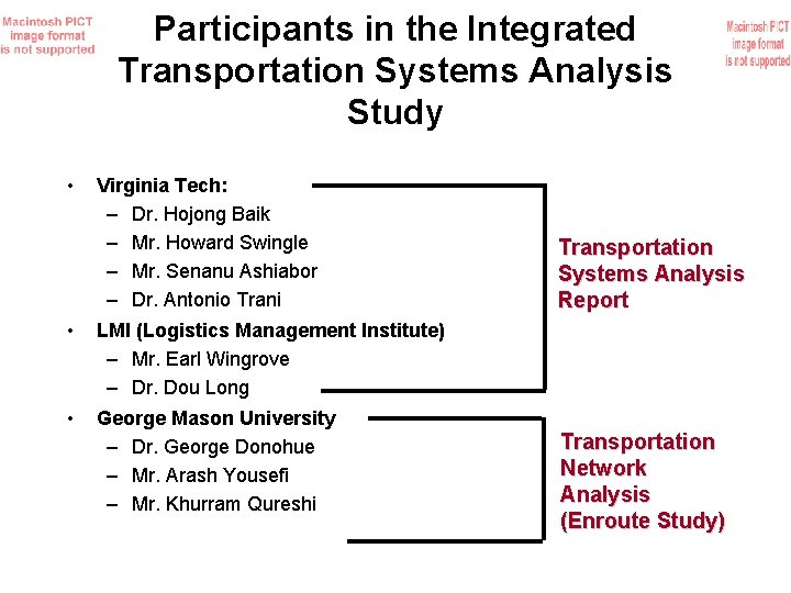
Participants in the Integrated Transportation Systems Analysis Study • Virginia Tech: – Dr. Hojong Baik – Mr. Howard Swingle – Mr. Senanu Ashiabor – Dr. Antonio Trani • LMI (Logistics Management Institute) – Mr. Earl Wingrove – Dr. Dou Long • George Mason University – Dr. George Donohue – Mr. Arash Yousefi – Mr. Khurram Qureshi Transportation Systems Analysis Report Transportation Network Analysis (Enroute Study)

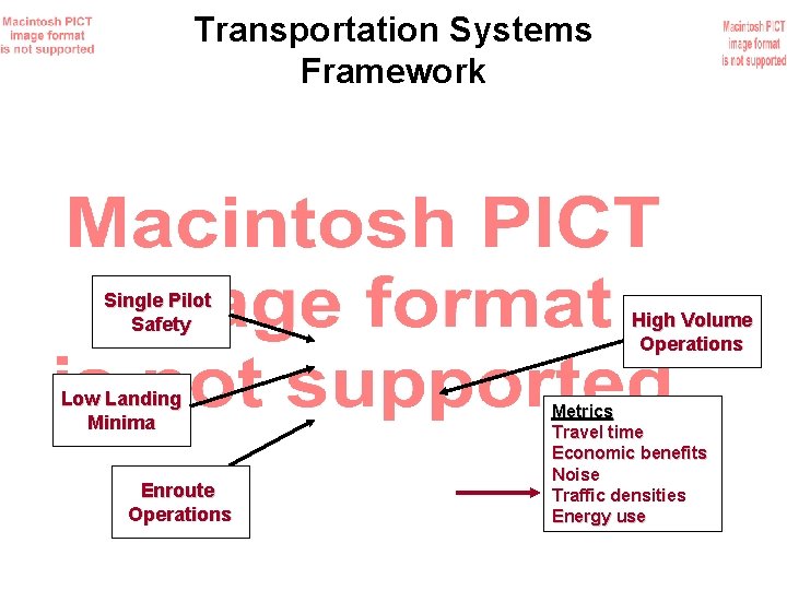
Transportation Systems Framework Single Pilot Safety Low Landing Minima Enroute Operations High Volume Operations Metrics Travel time Economic benefits Noise Traffic densities Energy use

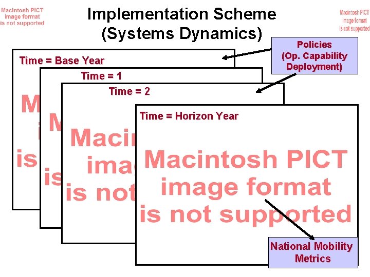
Implementation Scheme (Systems Dynamics) Time = Base Year Time = 1 Time = 2 Policies (Op. Capability Deployment) Time = Horizon Year National Mobility Metrics

Scenario Definition

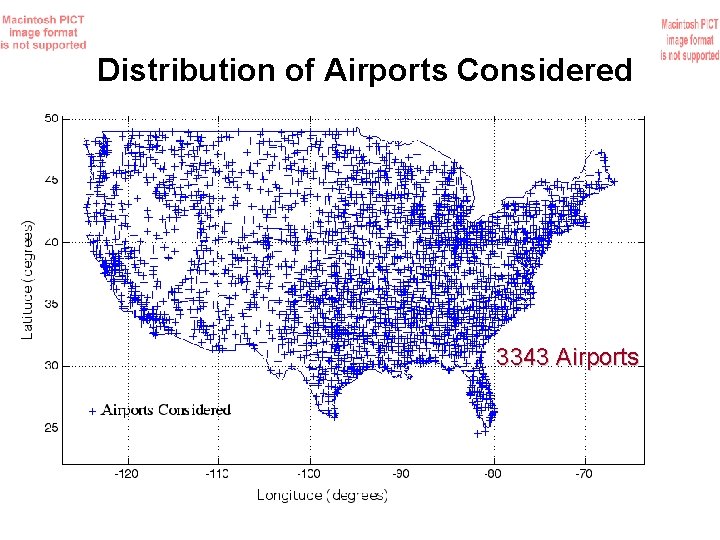
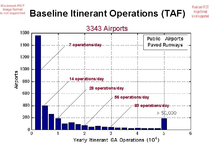
Distribution of Airports Considered 3343 Airports

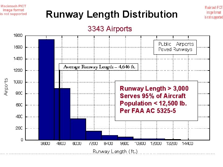
Runway Length Distribution 3343 Airports Runway Length > 3, 000 Serves 95% of Aircraft Population < 12, 500 lb. Per FAA AC 5325 -5

Baseline Itinerant Operations (TAF) 3343 Airports 7 operations/day 14 operations/day 28 operations/day 56 operations/day 83 operations/day

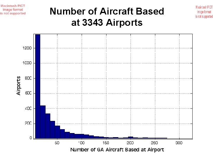
Number of Aircraft Based at 3343 Airports

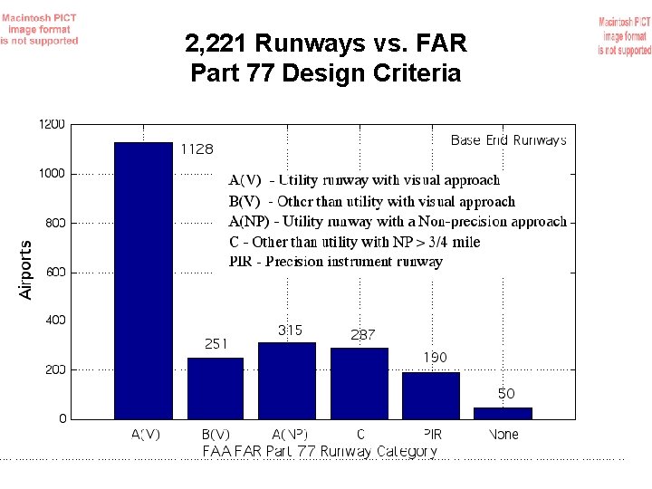
2, 221 Runways vs. FAR Part 77 Design Criteria

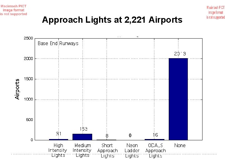
Approach Lights at 2, 221 Airports

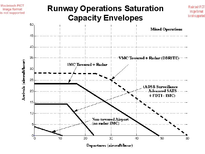
Runway Operations Saturation Capacity Envelopes

Where do People Live around Airports? 3346 Airports Towered Airports (474) Hub Airports (135) Large Hub Airports (30) Census 1990 and 2000 Data with 61, 224 tracts in NAS

Distribution of Income in the U. S. Percent of Population Census 2000 Data Household Income ($)

Travel Studies

The American Travel Survey Percent Travelers by Air (%) 540, 000 person trips 80, 000 households Household Income (105 $) One-Way Trip Distance (miles)

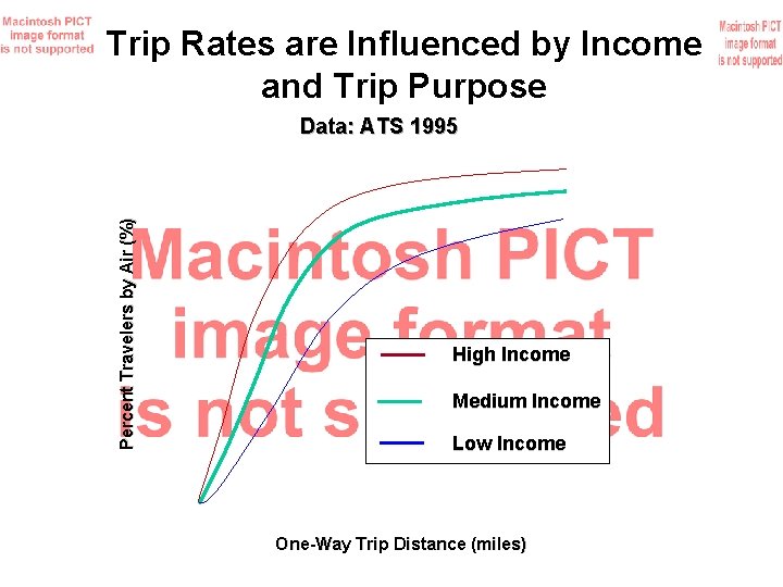
Trip Rates are Influenced by Income and Trip Purpose Percent Travelers by Air (%) Data: ATS 1995 High Income Medium Income Low Income One-Way Trip Distance (miles)

Transportation Systems Modeling

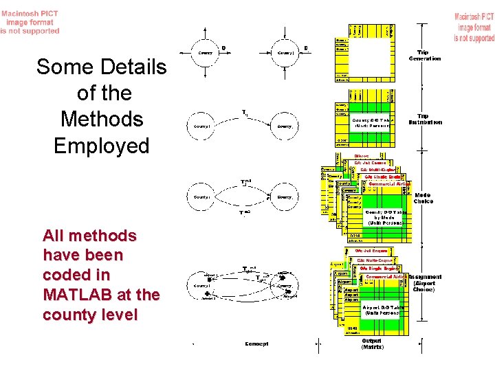
Some Details of the Methods Employed All methods have been coded in MATLAB at the county level

Trip Generation

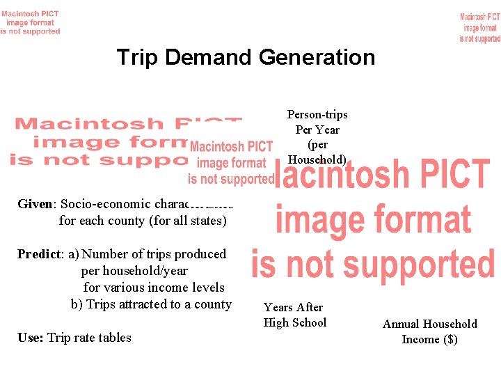
Trip Demand Generation Person-trips Per Year (per Household) Given: Socio-economic characteristics for each county (for all states) Predict: a) Number of trips produced per household/year for various income levels b) Trips attracted to a county Use: Trip rate tables Years After High School Annual Household Income ($)

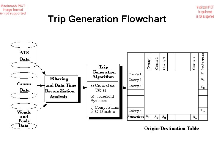
Trip Generation Flowchart

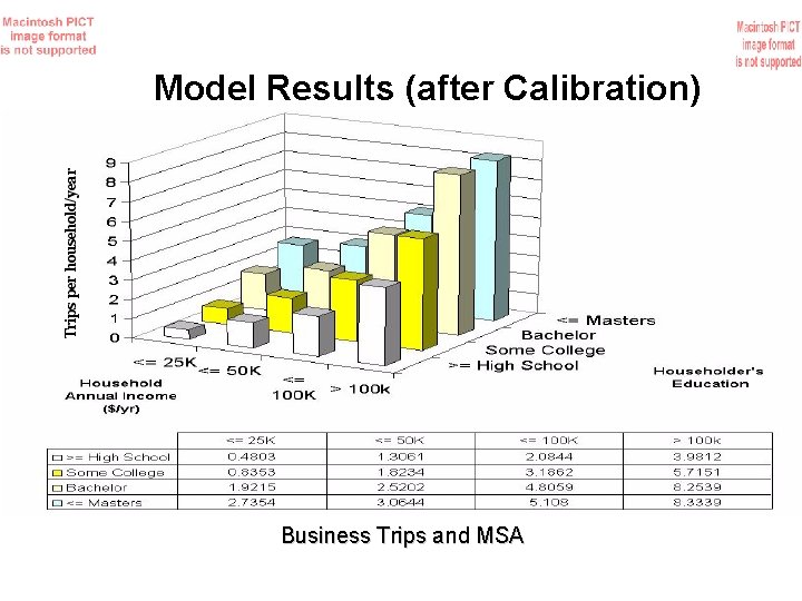
Model Results (after Calibration) Business Trips and MSA

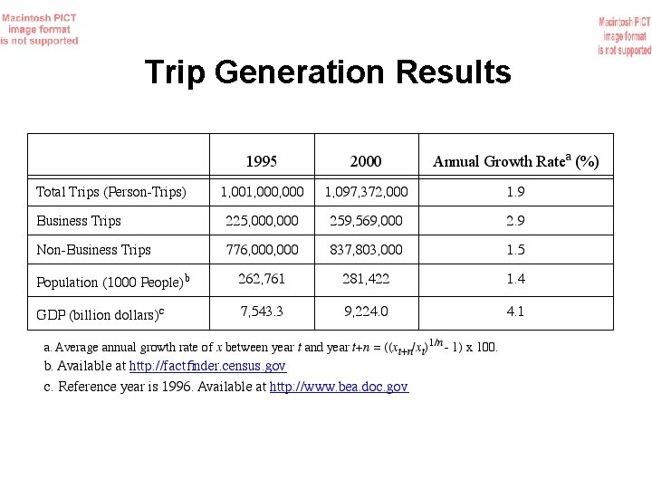
Trip Generation Results

Trip Distribution

Trip Distribution Analysis Given: Trips produced from and attracted to each county Predict: a) Number of person-trips from each origin to every destination (county to county) Use: Gravity Model

Trip Distribution Analysis • Calibration of Fij factors (impedence function) for business trips

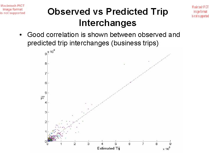
Observed vs Predicted Trip Interchanges • Good correlation is shown between observed and predicted trip interchanges (business trips)

Modal Split Analysis

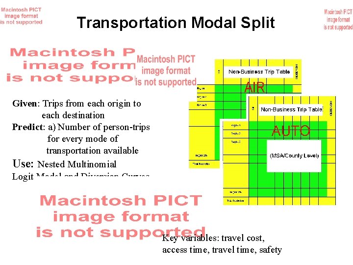
Transportation Modal Split Given: Trips from each origin to each destination Predict: a) Number of person-trips for every mode of transportation available Use: Nested Multinomial Logit Model and Diversion Curves Key variables: travel cost, access time, travel time, safety

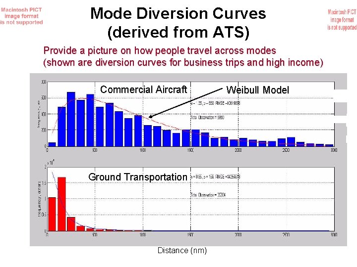
Mode Diversion Curves (derived from ATS) Provide a picture on how people travel across modes (shown are diversion curves for business trips and high income) Commercial Aircraft Ground Transportation Distance (nm) Weibull Model

Mode Diversion Curves (cont. ) Provide a picture on how people travel across modes (shown are diversion curves for business trips and high income) Ground Transportation General and Corporate Aviation Weibull Model Distance (nm)

Diversion Curves Represent Incomplete Information • Lack of understanding why traveler’s selected a mode • No information on mode attributes (i. e. , cost, convenience, perceived safety, etc. ) used by decision makers • No information on mode availability (i. e. who owns an aircraft or pilot capabilities - for GA trips) • Data set for GA and corporate travelers is small (as expected from the ATS sample size)

Recommended Next Steps (Modal Split Model) • Formulate a model split model that captures modespecific attributes and relates them to decisionmaker’s view in selecting a mode (Volpe is designing the experiment) • Calibrate the modal split model to include SATS as a feasible mode of transportation • The modal split model will be an unbiased model

Mode Split Model Development

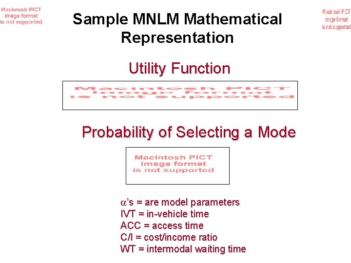
Sample MNLM Mathematical Representation Utility Function Probability of Selecting a Mode a’s = are model parameters IVT = in-vehicle time ACC = access time C/I = cost/income ratio WT = intermodal waiting time

Sample Use of the MNLM Results for a hypothetical 200 nm trip

Aircraft Cost Model • Quantifies all the operating costs of GA vehicles including future SATS aircraft (over the life cycle of the vehicle) • Critical sub-model in modal split analysis • Uses Business and Commercial Aviation Week database (Operations Planning Guide) • Use of regression analysis to derive various DOC and IOC factors

Aircraft Cost Model (Cost Categories Considered) • Variable costs (fuel, maintenance hrs. , parts, miscellaneous) • Fixed costs (hull insurance, liability, software, miscellaneous) • Periodic costs (engine overhaul, paint, interiors, flight deck upgrades) • Personnel costs (captain and first officer - if applicable) • Training costs (crew training and recurrent training, maintenance training) • Facilities costs (hangar space, office lease, miscellaneous) • Depreciation cost (amortization of aircraft value)

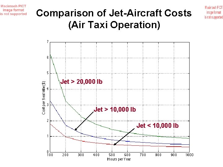
Small Aircraft Cost Model • Uses real-data bases collected by Business and Commercial Aviation and ARG/US • Employs regression models to derive realistic operation costs for Piston, Turboprop and Jet-engine powered aircraft 600 hours / year Jet Aircraft

Comparison of Jet-Aircraft Costs (Air Taxi Operation) Jet > 20, 000 lb Jet > 10, 000 lb Jet < 10, 000 lb

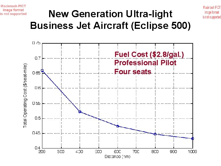
Total Operating Cost ($/seat-mile) New Generation Ultra-light Business Jet Aircraft (Eclipse 500) Fuel Cost ($2. 8/gal. ) Professional Pilot Four seats

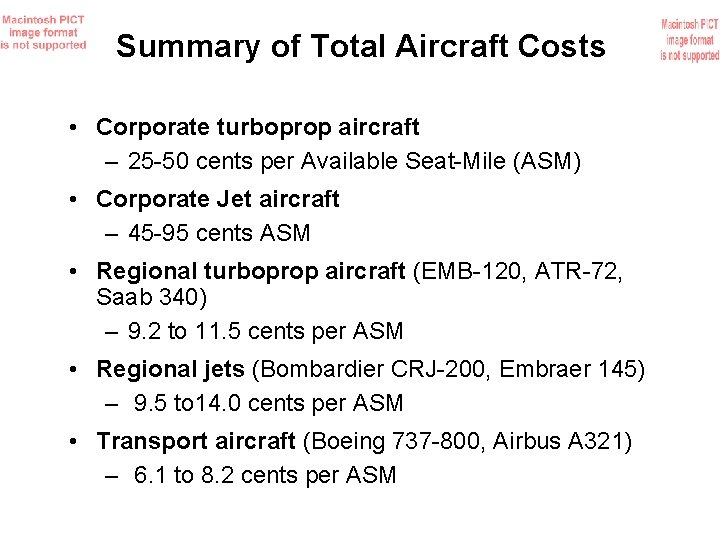
Summary of Total Aircraft Costs • Corporate turboprop aircraft – 25 -50 cents per Available Seat-Mile (ASM) • Corporate Jet aircraft – 45 -95 cents ASM • Regional turboprop aircraft (EMB-120, ATR-72, Saab 340) – 9. 2 to 11. 5 cents per ASM • Regional jets (Bombardier CRJ-200, Embraer 145) – 9. 5 to 14. 0 cents per ASM • Transport aircraft (Boeing 737 -800, Airbus A 321) – 6. 1 to 8. 2 cents per ASM

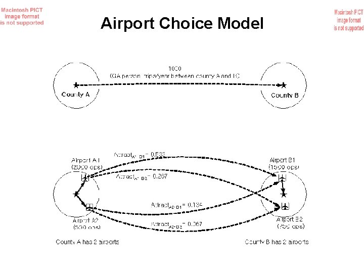
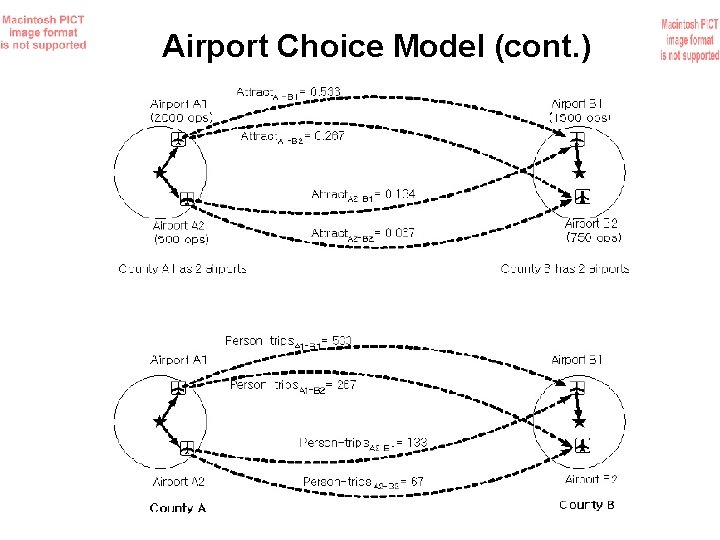
Airport Choice Modeling • The goal is to distribute trip interchanges across all selected airports • Currently we modeled 3, 343 GA and hub airports

Airport Choice Model (Attractiveness Parameters)

Airport Choice Model

Airport Choice Model (cont. )

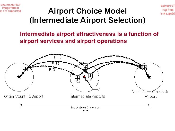
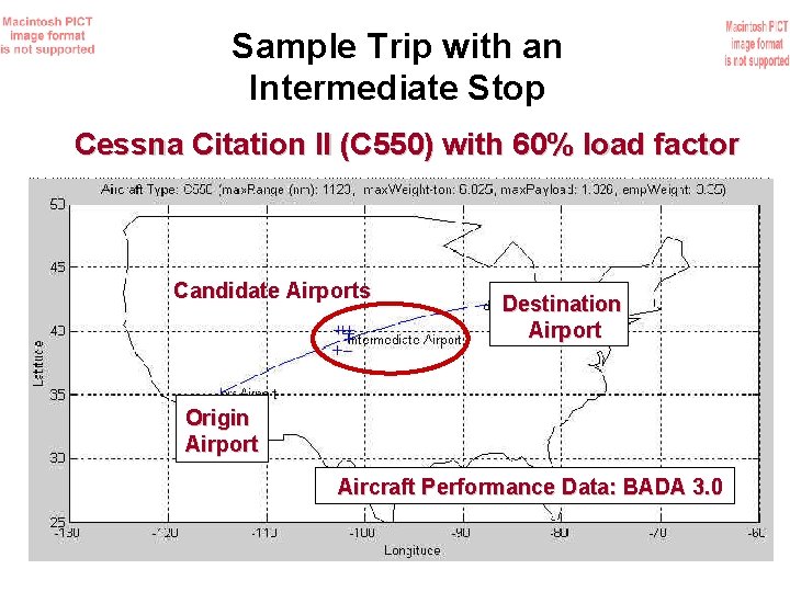
Airport Choice Model (Intermediate Airport Selection) Intermediate airport attractiveness is a function of airport services and airport operations

Sample Trip with an Intermediate Stop Cessna Citation II (C 550) with 60% load factor Candidate Airports Destination Airport Origin Airport Aircraft Performance Data: BADA 3. 0

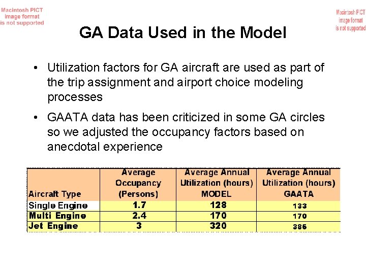
GA Data Used in the Model • Utilization factors for GA aircraft are used as part of the trip assignment and airport choice modeling processes • GAATA data has been criticized in some GA circles so we adjusted the occupancy factors based on anecdotal experience

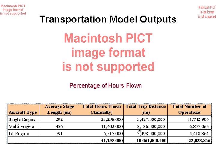
Transportation Model Outputs Percentage of Hours Flown

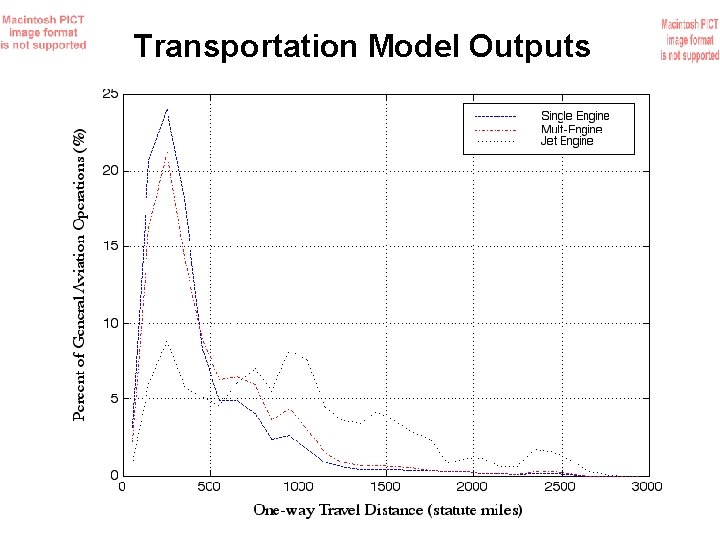
Transportation Model Outputs

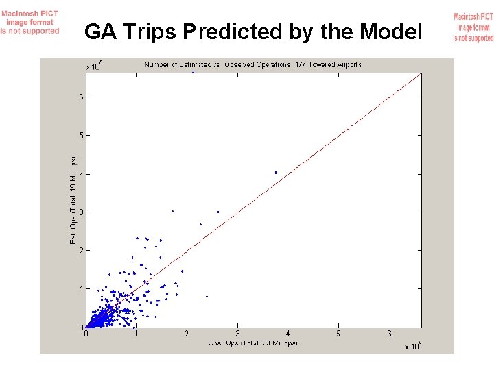
GA Trips Predicted by the Model

Transportation Network Analysis

Transportation Network Analysis

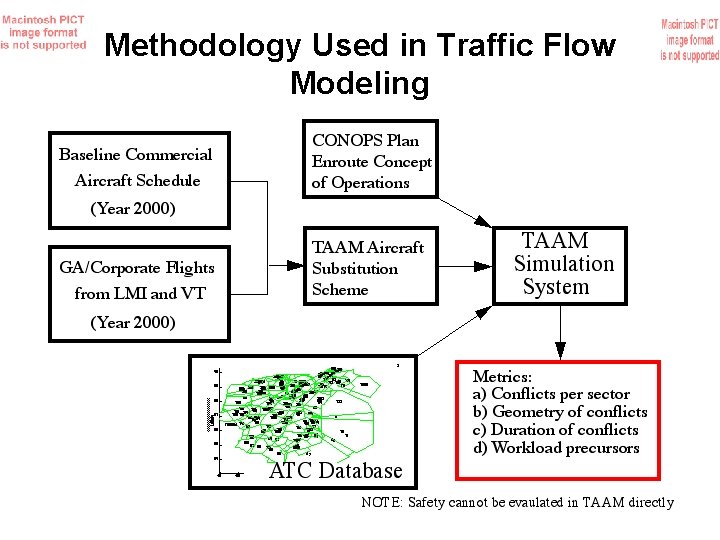
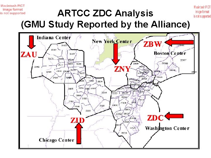
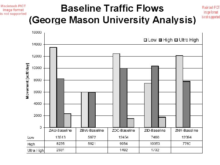
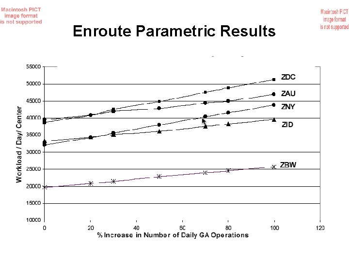
Network Scenario Analysis • Used fast-time simulation models – TAAM – LMI SATS Net – Flight explorer • 29, 815 aircraft modeled in TAAM (single day operations at 5 ARTCC Centers) – Included all airline traffic – Included all GA traffic (estimated from our transportation systems analysis method) • Derived precursor metrics of workload and sector delays

Methodology Used in Traffic Flow Modeling

ARTCC ZDC Analysis (GMU Study Reported by the Alliance)

Baseline Traffic Flows (George Mason University Analysis)

Enroute Parametric Results

Enroute Conflict Analysis (Baik et al. , 2002) Number of Daily Conflicts Region of Interest = Size of ZDC ARTCC Number of Daily Flights (all types)

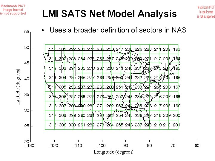
LMI SATS Net Model Analysis • Uses a broader definition of sectors in NAS

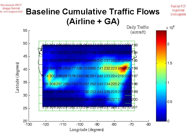
Baseline Cumulative Traffic Flows (Airline + GA)

Animation of Baseline NAS Flows

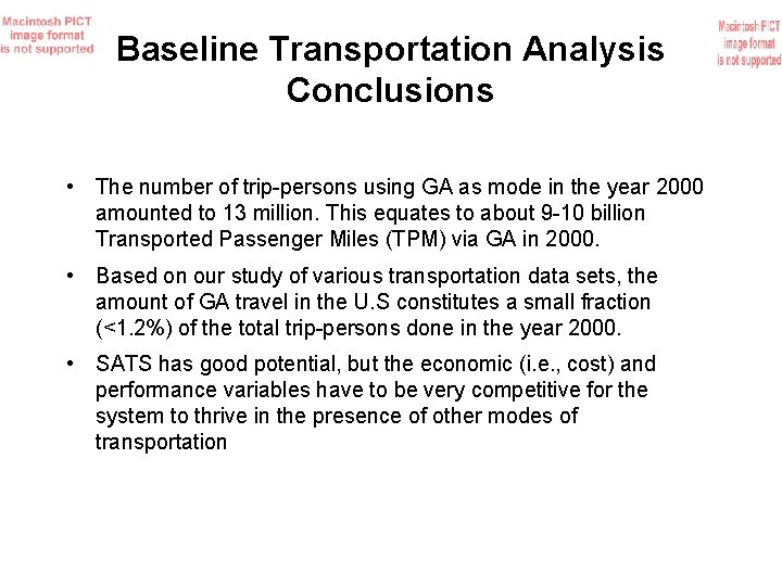
Baseline Transportation Analysis Conclusions • The number of trip-persons using GA as mode in the year 2000 amounted to 13 million. This equates to about 9 -10 billion Transported Passenger Miles (TPM) via GA in 2000. • Based on our study of various transportation data sets, the amount of GA travel in the U. S constitutes a small fraction (<1. 2%) of the total trip-persons done in the year 2000. • SATS has good potential, but the economic (i. e. , cost) and performance variables have to be very competitive for the system to thrive in the presence of other modes of transportation

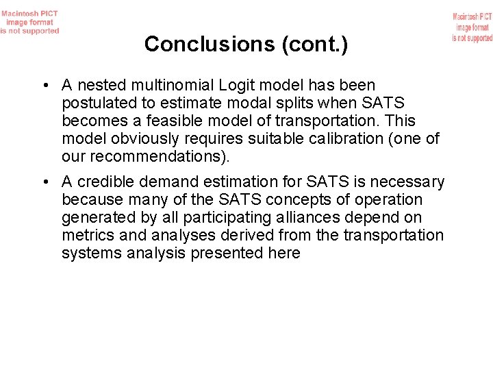
Conclusions (cont. ) • A nested multinomial Logit model has been postulated to estimate modal splits when SATS becomes a feasible model of transportation. This model obviously requires suitable calibration (one of our recommendations). • A credible demand estimation for SATS is necessary because many of the SATS concepts of operation generated by all participating alliances depend on metrics and analyses derived from the transportation systems analysis presented here

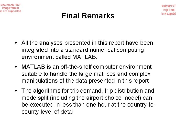
Final Remarks • All the analyses presented in this report have been integrated into a standard numerical computing environment called MATLAB. • MATLAB is an off-the-shelf computer environment suitable to handle the large matrices and complex manipulations of the data presented in this report • The algorithms for trip demand, trip distribution and mode split (including the airport choice model) can be executed in less than one hour at the country-tocounty level of detail

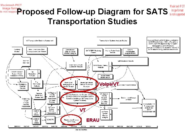
Proposed Follow-up Diagram for SATS Transportation Studies Volpe/VT VT ERAU