
SASSTAT LECTURE 1 pgrebennikovibs ru Copyright 2013 SAS
SAS/STAT LECTURE 1 ВВЕДЕНИЕ. ДИСПЕРСИОННЫЙ АНАЛИЗ Павел Гребенников pgrebennikov@ibs. ru Copyright © 2013, SAS Institute Inc. All rights reserved.
SAS/STAT ОБЗОР КУРСА • • ANOVA – дисперсионный анализ LINEAR REGRESSION – линейная регрессия LOGISTIC REGRESSION – логистическая регрессия Generalized LM – обобщенные линейные модели • POISSON REGRESSION & ZERO-INFLATED POISSON • NEGATIVE BINOMIAL REGRESSION • GAMMA REGRESSION Copyright © 2013, SAS Institute Inc. All rights reserved.

ПОМОЩЬ Copyright © 2013, SAS Institute Inc. All rights reserved.
SAS/STAT ГДЕ ИСКАТЬ ПОМОЩИ…. • HTTP: //SUPPORT. SAS. COM/DOCUMENTATION/ONLINEDOC/STAT/INDEX. HTML • HTTP: //WWW. MACHINELEARNING. RU • HTTP: //STANFORD. EDU/ • HTTPS: //WWW. GOOGLE. RU/ • HTTP: //EN. WIKIPEDIA. ORG/WIKI/ANALYSIS_OF_VARIANCE Copyright © 2013, SAS Institute Inc. All rights reserved.

ДИСПЕРСИОННЫЙ АНАЛИЗ Copyright © 2013, SAS Institute Inc. All rights reserved.
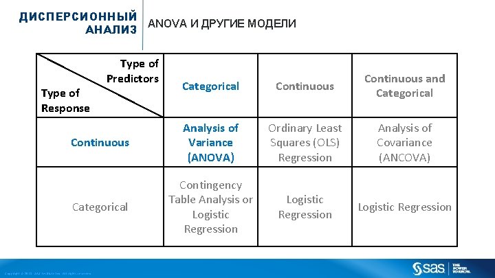
ДИСПЕРСИОННЫЙ ANOVA И ДРУГИЕ МОДЕЛИ АНАЛИЗ Type of Predictors Categorical Continuous and Categorical Continuous Analysis of Variance (ANOVA) Ordinary Least Squares (OLS) Regression Analysis of Covariance (ANCOVA) Categorical Contingency Table Analysis or Logistic Regression Type of Response Copyright © 2013, SAS Institute Inc. All rights reserved.
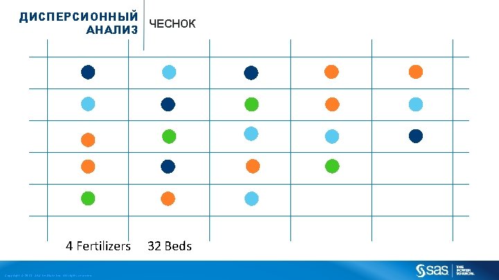
ДИСПЕРСИОННЫЙ ЧЕСНОК АНАЛИЗ 4 Fertilizers Copyright © 2013, SAS Institute Inc. All rights reserved. 32 Beds
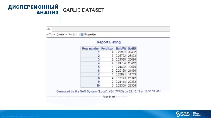
ДИСПЕРСИОННЫЙ GARLIC DATASET АНАЛИЗ Copyright © 2013, SAS Institute Inc. All rights reserved.
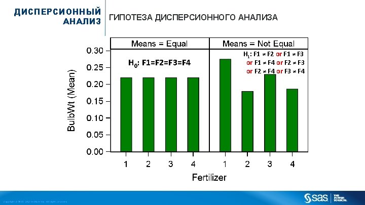
ДИСПЕРСИОННЫЙ ГИПОТЕЗА ДИСПЕРСИОННОГО АНАЛИЗА АНАЛИЗ H 0: F 1=F 2=F 3=F 4 Copyright © 2013, SAS Institute Inc. All rights reserved. H 1: F 1 ≠ F 2 or F 1 ≠ F 3 or F 1 ≠ F 4 or F 2 ≠ F 3 or F 2 ≠ F 4 or F 3 ≠ F 4
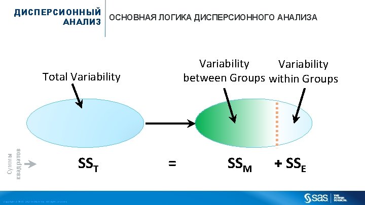
ДИСПЕРСИОННЫЙ ОСНОВНАЯ ЛОГИКА ДИСПЕРСИОННОГО АНАЛИЗА АНАЛИЗ Variability between Groups within Groups Суммы квадратов Total Variability Copyright © 2013, SAS Institute Inc. All rights reserved. SST = SSM + SSE
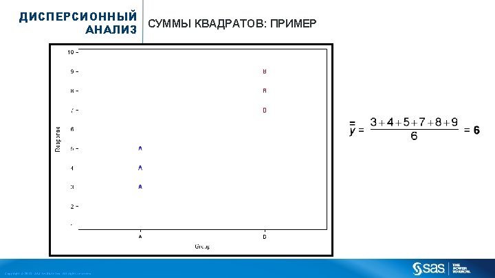
ДИСПЕРСИОННЫЙ СУММЫ КВАДРАТОВ: ПРИМЕР АНАЛИЗ Copyright © 2013, SAS Institute Inc. All rights reserved.
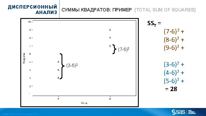
ДИСПЕРСИОННЫЙ СУММЫ КВАДРАТОВ: ПРИМЕР [TOTAL SUM OF SQUARES] АНАЛИЗ SST = (7 -6)2 (3 -6)2 Copyright © 2013, SAS Institute Inc. All rights reserved. (7 -6)2 + (8 -6)2 + (9 -6)2 + (3 -6)2 + (4 -6)2 + (5 -6)2 + = 28
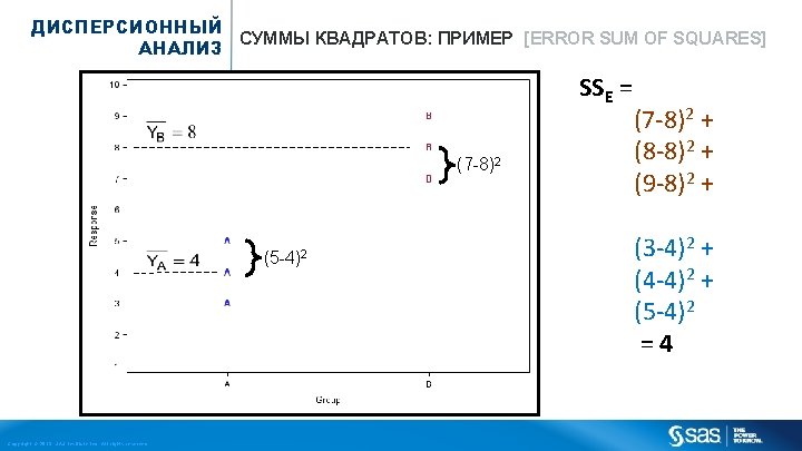
ДИСПЕРСИОННЫЙ СУММЫ КВАДРАТОВ: ПРИМЕР [ERROR SUM OF SQUARES] АНАЛИЗ SSE = (7 -8)2 (5 -4)2 Copyright © 2013, SAS Institute Inc. All rights reserved. (7 -8)2 + (8 -8)2 + (9 -8)2 + (3 -4)2 + (4 -4)2 + (5 -4)2 =4
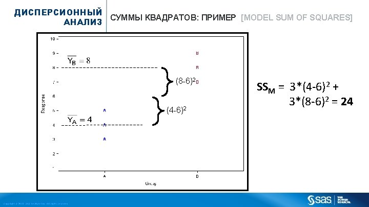
ДИСПЕРСИОННЫЙ СУММЫ КВАДРАТОВ: ПРИМЕР [MODEL SUM OF SQUARES] АНАЛИЗ (8 -6)2 (4 -6)2 Copyright © 2013, SAS Institute Inc. All rights reserved. SSM = 3*(4 -6)2 + 3*(8 -6)2 = 24
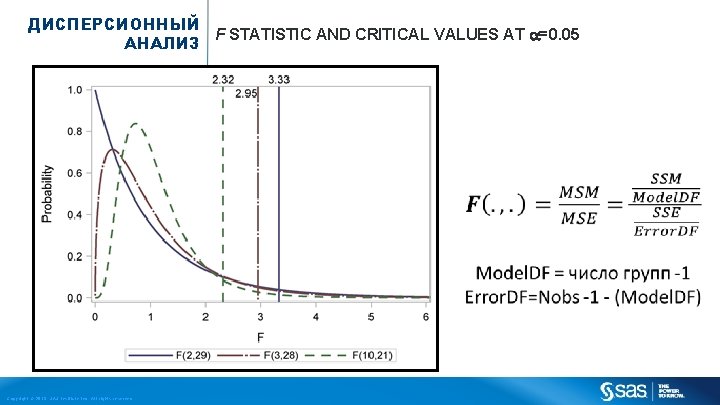
ДИСПЕРСИОННЫЙ F STATISTIC AND CRITICAL VALUES AT =0. 05 АНАЛИЗ Copyright © 2013, SAS Institute Inc. All rights reserved.
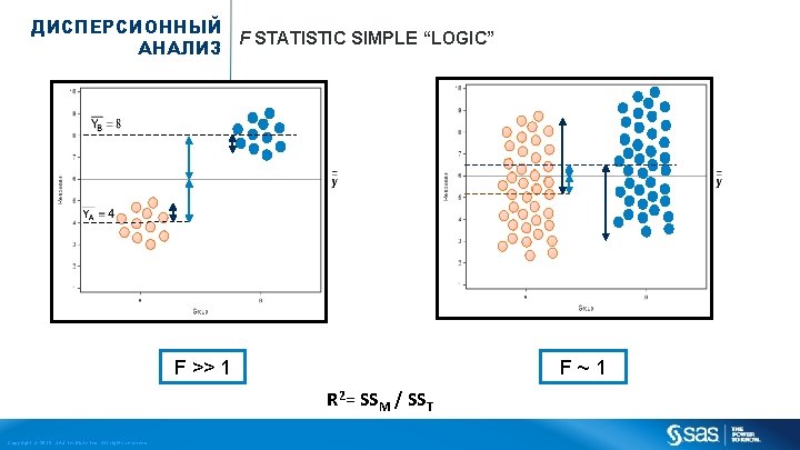
ДИСПЕРСИОННЫЙ F STATISTIC SIMPLE “LOGIC” АНАЛИЗ F >> 1 F ~ 1 R 2= SSM / SST Copyright © 2013, SAS Institute Inc. All rights reserved.
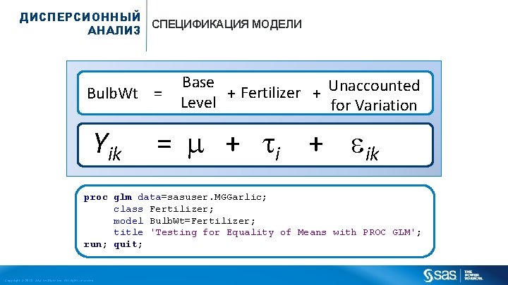
ДИСПЕРСИОННЫЙ СПЕЦИФИКАЦИЯ МОДЕЛИ АНАЛИЗ Bulb. Wt = Yik Base + Fertilizer + Unaccounted Level for Variation = + ik proc glm data=sasuser. MGGarlic; class Fertilizer; model Bulb. Wt=Fertilizer; title 'Testing for Equality of Means with PROC GLM'; run; quit; Copyright © 2013, SAS Institute Inc. All rights reserved.
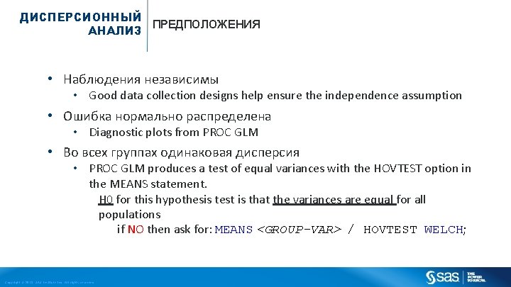
ДИСПЕРСИОННЫЙ ПРЕДПОЛОЖЕНИЯ АНАЛИЗ • Наблюдения независимы • Good data collection designs help ensure the independence assumption • Ошибка нормально распределена • Diagnostic plots from PROC GLM • Во всех группах одинаковая дисперсия • PROC GLM produces a test of equal variances with the HOVTEST option in the MEANS statement. H 0 for this hypothesis test is that the variances are equal for all populations if NO then ask for: MEANS <GROUP-VAR> / HOVTEST WELCH; Copyright © 2013, SAS Institute Inc. All rights reserved.
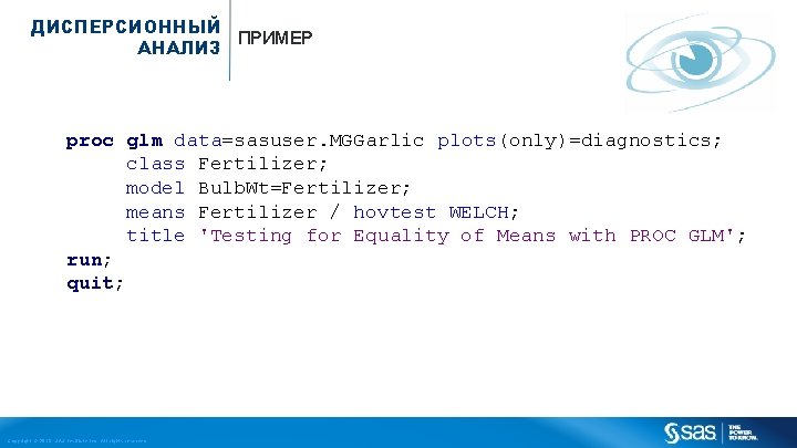
ДИСПЕРСИОННЫЙ ПРИМЕР АНАЛИЗ proc glm data=sasuser. MGGarlic plots(only)=diagnostics; class Fertilizer; model Bulb. Wt=Fertilizer; means Fertilizer / hovtest WELCH; title 'Testing for Equality of Means with PROC GLM'; run; quit; Copyright © 2013, SAS Institute Inc. All rights reserved.
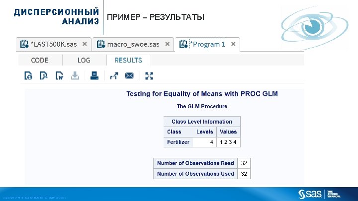
ДИСПЕРСИОННЫЙ ПРИМЕР – РЕЗУЛЬТАТЫ АНАЛИЗ Copyright © 2013, SAS Institute Inc. All rights reserved.
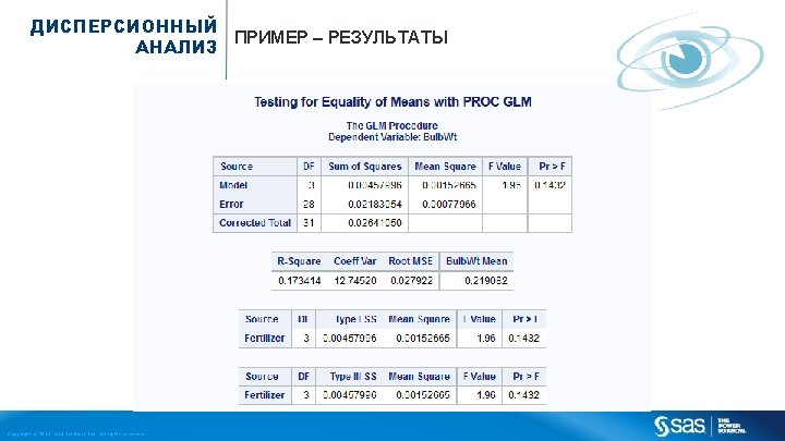
ДИСПЕРСИОННЫЙ ПРИМЕР – РЕЗУЛЬТАТЫ АНАЛИЗ Copyright © 2013, SAS Institute Inc. All rights reserved.
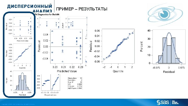
ДИСПЕРСИОННЫЙ ПРИМЕР – РЕЗУЛЬТАТЫ АНАЛИЗ Copyright © 2013, SAS Institute Inc. All rights reserved.
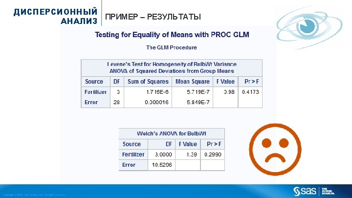
ДИСПЕРСИОННЫЙ ПРИМЕР – РЕЗУЛЬТАТЫ АНАЛИЗ Copyright © 2013, SAS Institute Inc. All rights reserved.
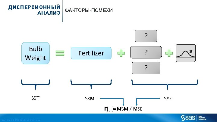
ДИСПЕРСИОННЫЙ ФАКТОРЫ-ПОМЕХИ АНАЛИЗ ? Bulb Weight ? Fertilizer ? SST SSM SSE F( , )=MSM / MSE Copyright © 2013, SAS Institute Inc. All rights reserved.
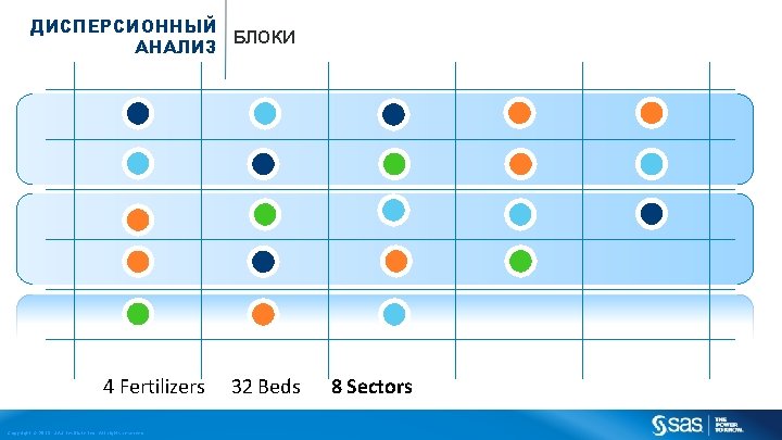
ДИСПЕРСИОННЫЙ БЛОКИ АНАЛИЗ 4 Fertilizers Copyright © 2013, SAS Institute Inc. All rights reserved. 32 Beds 8 Sectors
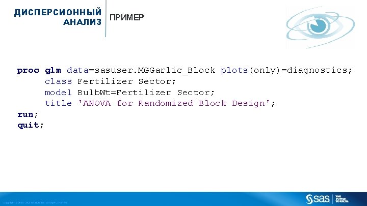
ДИСПЕРСИОННЫЙ ПРИМЕР АНАЛИЗ proc glm data=sasuser. MGGarlic_Block plots(only)=diagnostics; class Fertilizer Sector; model Bulb. Wt=Fertilizer Sector; title 'ANOVA for Randomized Block Design'; run; quit; Copyright © 2013, SAS Institute Inc. All rights reserved.
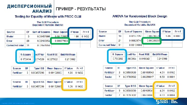
ДИСПЕРСИОННЫЙ ПРИМЕР - РЕЗУЛЬТАТЫ АНАЛИЗ Copyright © 2013, SAS Institute Inc. All rights reserved.
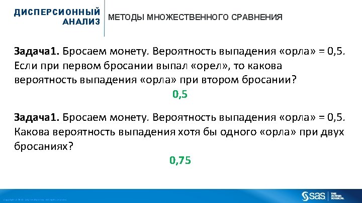
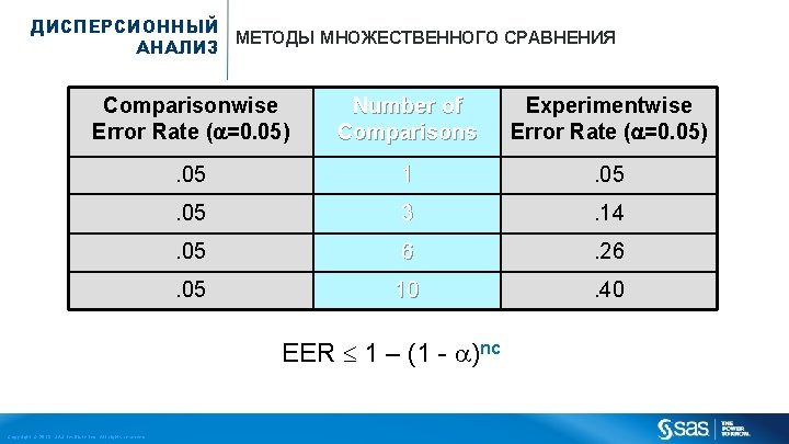
ДИСПЕРСИОННЫЙ МЕТОДЫ МНОЖЕСТВЕННОГО СРАВНЕНИЯ АНАЛИЗ Comparisonwise Error Rate ( =0. 05) Number of Comparisons Experimentwise Error Rate ( =0. 05) . 05 1 . 05 3 . 14 . 05 6 . 26 . 05 10 . 40 EER 1 – (1 - )nc Copyright © 2013, SAS Institute Inc. All rights reserved.
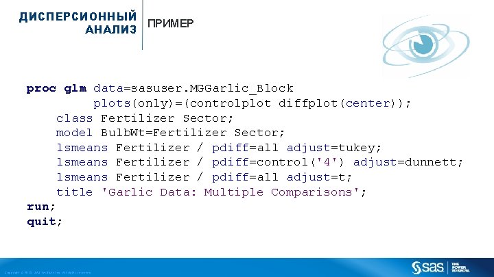
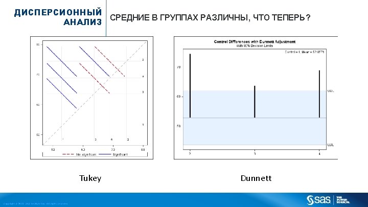
ДИСПЕРСИОННЫЙ ПРИМЕР АНАЛИЗ proc glm data=sasuser. MGGarlic_Block plots(only)=(controlplot diffplot(center)); class Fertilizer Sector; model Bulb. Wt=Fertilizer Sector; lsmeans Fertilizer / pdiff=all adjust=tukey; lsmeans Fertilizer / pdiff=control('4') adjust=dunnett; lsmeans Fertilizer / pdiff=all adjust=t; title 'Garlic Data: Multiple Comparisons'; run; quit; Copyright © 2013, SAS Institute Inc. All rights reserved.
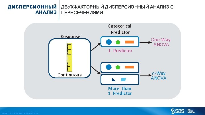
ДИСПЕРСИОННЫЙ ДВУХФАКТОРНЫЙ ДИСПЕРСИОННЫЙ АНАЛИЗ С АНАЛИЗ ПЕРЕСЕЧЕНИЯМИ Response Categorical Predictor 1 Predictor n-Way ANOVA Continuous More than 1 Predictor Copyright © 2013, SAS Institute Inc. All rights reserved. One-Way ANOVA
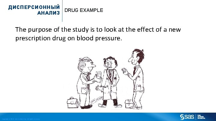
ДИСПЕРСИОННЫЙ DRUG EXAMPLE АНАЛИЗ The purpose of the study is to look at the effect of a new prescription drug on blood pressure. Copyright © 2013, SAS Institute Inc. All rights reserved.
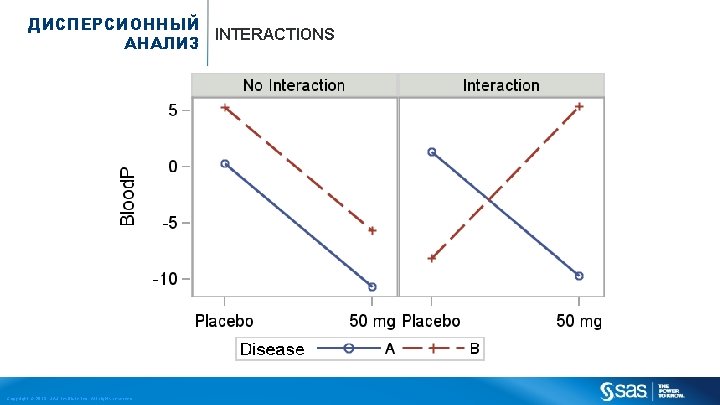
ДИСПЕРСИОННЫЙ INTERACTIONS АНАЛИЗ Copyright © 2013, SAS Institute Inc. All rights reserved.
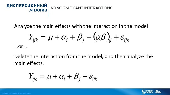
ДИСПЕРСИОННЫЙ NONSIGNIFICANT INTERACTIONS АНАЛИЗ Analyze the main effects with the interaction in the model. …or… Delete the interaction from the model, and then analyze the main effects. Copyright © 2013, SAS Institute Inc. All rights reserved.
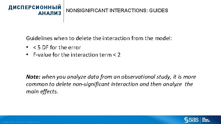
ДИСПЕРСИОННЫЙ NONSIGNIFICANT INTERACTIONS: GUIDES АНАЛИЗ Guidelines when to delete the interaction from the model: • < 5 DF for the error • F-value for the interaction term < 2 Note: when you analyze data from an observational study, it is more common to delete non-significant interaction and then analyze the main effects. Copyright © 2013, SAS Institute Inc. All rights reserved.
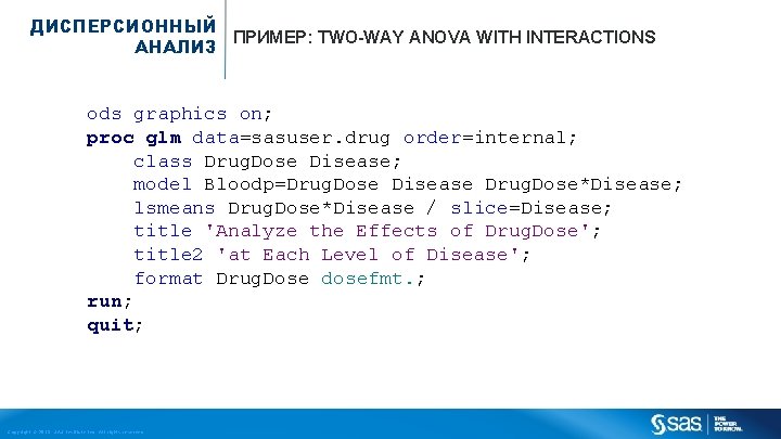
ДИСПЕРСИОННЫЙ ПРИМЕР: TWO-WAY ANOVA WITH INTERACTIONS АНАЛИЗ ods graphics on; proc glm data=sasuser. drug order=internal; class Drug. Dose Disease; model Bloodp=Drug. Dose Disease Drug. Dose*Disease; lsmeans Drug. Dose*Disease / slice=Disease; title 'Analyze the Effects of Drug. Dose'; title 2 'at Each Level of Disease'; format Drug. Dose dosefmt. ; run; quit; Copyright © 2013, SAS Institute Inc. All rights reserved.
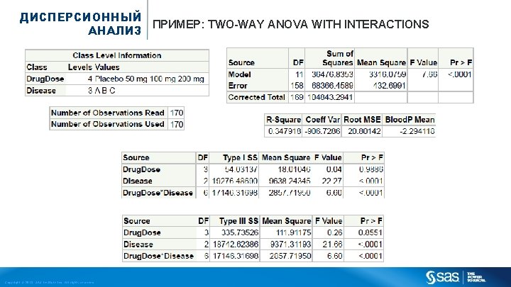
ДИСПЕРСИОННЫЙ ПРИМЕР: TWO-WAY ANOVA WITH INTERACTIONS АНАЛИЗ Copyright © 2013, SAS Institute Inc. All rights reserved.
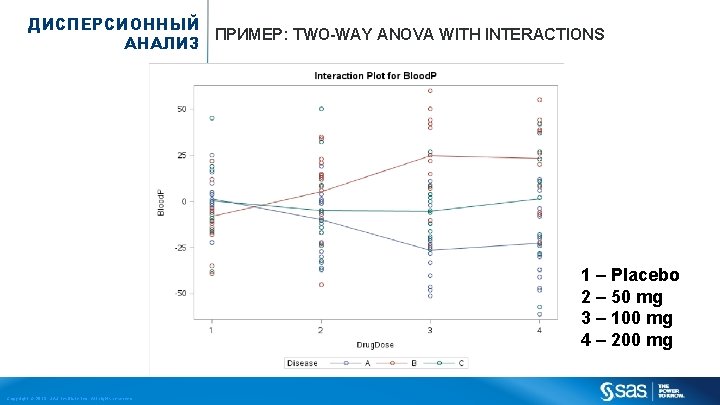
ДИСПЕРСИОННЫЙ ПРИМЕР: TWO-WAY ANOVA WITH INTERACTIONS АНАЛИЗ 1 – Placebo 2 – 50 mg 3 – 100 mg 4 – 200 mg Copyright © 2013, SAS Institute Inc. All rights reserved.
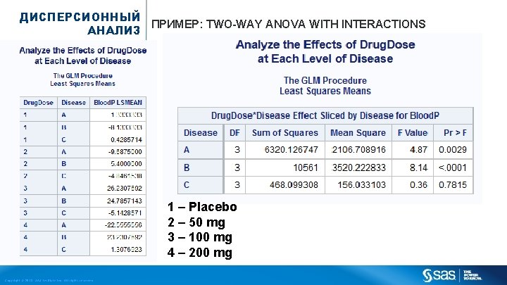
ДИСПЕРСИОННЫЙ ПРИМЕР: TWO-WAY ANOVA WITH INTERACTIONS АНАЛИЗ 1 – Placebo 2 – 50 mg 3 – 100 mg 4 – 200 mg Copyright © 2013, SAS Institute Inc. All rights reserved.

HOME WORK Copyright © 2013, SAS Institute Inc. All rights reserved.
- Slides: 46