Sampling Fluctuations and Their Contribution to Hadron Energy

Sampling Fluctuations and Their Contribution to Hadron Energy Resolution A. Para, February 20, 2007

Motivation n Homogenous calorimeter with dual readout (Cherenkov + ionization) offers a prospect of high resolution hadron calorimetry. Natural implementation of a dual readout concept: two-component calorimeter (for example lead glass/scintillator). In such a calorimeter both components are sampled, hence undergo sampling fluctuations The target energy resolution is very good, hence the contribution of sampling fluctuations must be well understood.

Goal n Develop a phenomenological model of contribution of sampling fluctuations to the hadron energy resolution as a function of the detector geometry: sampling frequency (absorber thickness) and the active detector thickness.

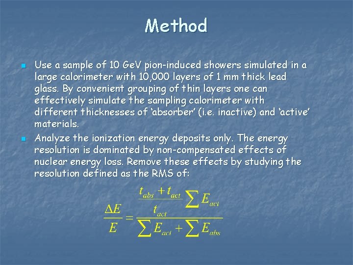
Method n n Use a sample of 10 Ge. V pion-induced showers simulated in a large calorimeter with 10, 000 layers of 1 mm thick lead glass. By convenient grouping of thin layers one can effectively simulate the sampling calorimeter with different thicknesses of ‘absorber’ (i. e. inactive) and ‘active’ materials. Analyze the ionization energy deposits only. The energy resolution is dominated by non-compensated effects of nuclear energy loss. Remove these effects by studying the resolution defined as the RMS of:

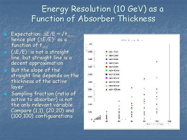
Energy Resolution (10 Ge. V) as a Function of Absorber Thickness n n Expectation: DE/E ~ √tabs, hence plot (DE/E)2 as a function of tabs (DE/E)2 is not a straight line, but straight line is a decent approximation But the slope of the straight line depends on the thickness of the active layer Sampling fraction (ratio of active to absorber) is not the only relevant variable. Compare (1, 1), (20, 20) and (100, 100) configuarations

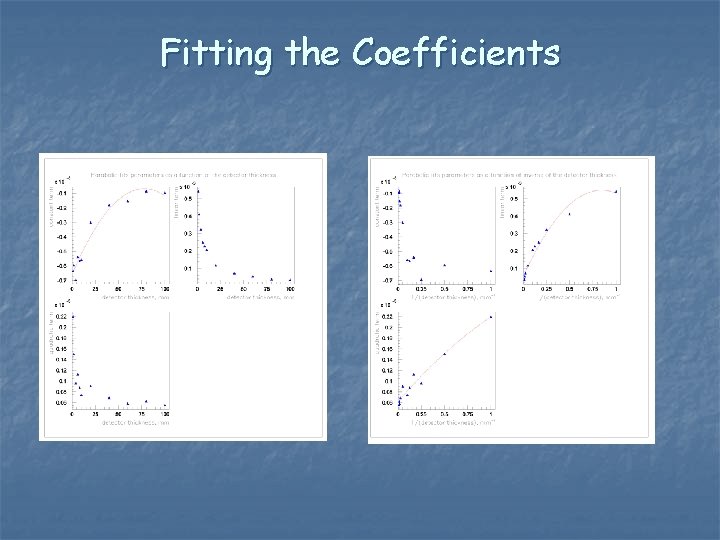
Strategy n n The previous plot is too busy to analyze. Try to find an effective description in three steps: n Fit (DE/E)2 as a quadratic function of tabs (green line in the forthcoming plots) n Parameterize the coefficients (constant, linear and quadratic term) as a quadratic function of the tact (or 1/tact) n Parameterize (red line in the forthcoming plots): n (DE/E)2(tabs, tact) = A(tact)tabs 2 + B(tact)tabs +C(tact) Note: the above ansatz is a crude guess. Fitting separate coefficients is not a good recipe, as they are usually correlated. It may not work very well. Better approximations can be found.

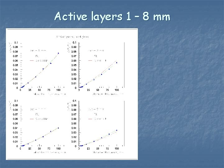
Active layers 1 – 8 mm

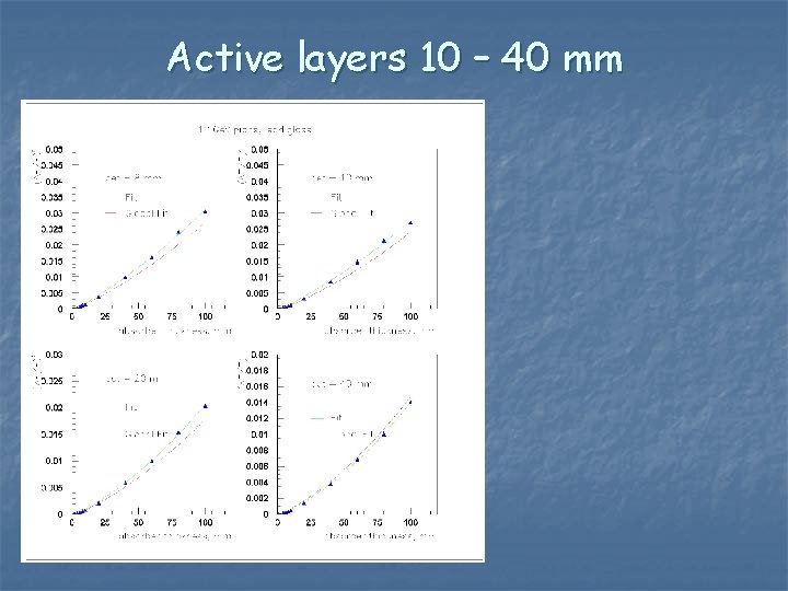
Active layers 10 – 40 mm

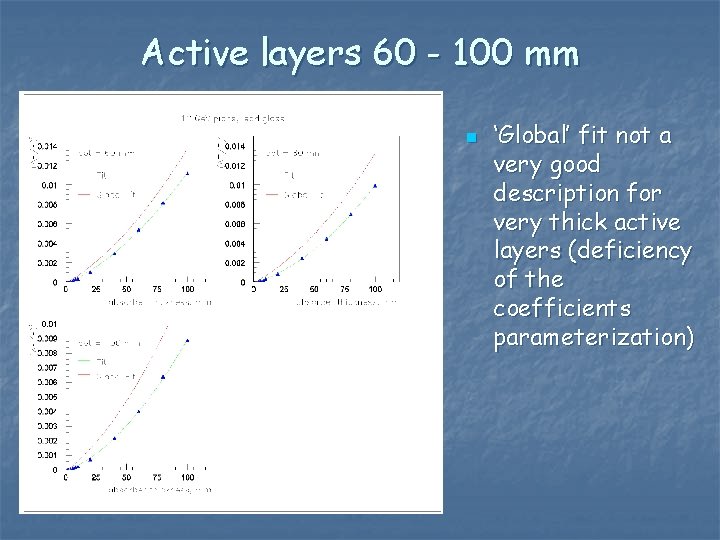
Active layers 60 - 100 mm n ‘Global’ fit not a very good description for very thick active layers (deficiency of the coefficients parameterization)

Fitting the Coefficients

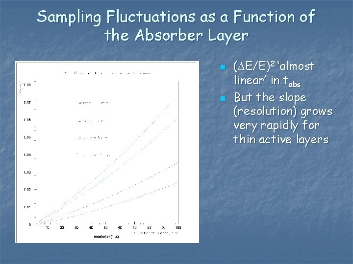
Sampling Fluctuations as a Function of the Absorber Layer n n (DE/E)2 ‘almost linear’ in tabs But the slope (resolution) grows very rapidly for thin active layers